
Computational Resource Optimisation in Feature Selection under Class Imbalance Conditions
Abstract
Feature selection is crucial for reducing data dimensionality as well as enhancing model interpretability and performance in machine learning tasks. However, selecting the most informative features in large dataset often incurs high computational costs. This study explores the possibility of performing feature selection on a subset of data to reduce the computational burden. The study uses five real-life datasets with substantial sample sizes and severe class imbalance ratios between 0.09 – 0.18. The results illustrate the variability of feature importance with smaller sample fractions in different models. In this cases considered, light gradient-boosting machine exhibited the least variability, even with reduced sample fractions, while also incurring the least computational resource.
1Introduction
In the development of prediction models for real-world applications, two key challenges often arise: high-dimensionality resulting from the numerous features, and class-imbalance due to the rarity of samples in the positive class. Feature selection methods are utilized to address issues of high-dimensionality by selecting a smaller subset of relevant features, thus reducing noise, increasing interpretability, and enhancing model performance Cai et al., 2018Dhal & Azad, 2022Udu et al., 2023.
Studies Yin et al., 2013Tsai & Sung, 2020Haro-García et al., 2020Matharaarachchi et al., 2021 on the performance of feature selection methods with class imbalance data have been undertaken on using synthetic and real-life datasets. A significant drawback noted was the computational cost of their approach on large sample sizes. While experimental investigations of feature selection amid class imbalance conditions have been studied in the literature, there is a need to further understand the effect of sample size on performance degradation of feature selection methods. This would offer valuable insights into tackling the associated resource expense involved in undertaking feature selection with respect to large sample sizes where class-imbalance exists, for a wide range of applications.
This study investigates the impact of performing feature selection on a reduced dataset on feature importance and model performance, using five real-life datasets characterised by large sample sizes and severe class imbalance structures. We employ a feature selection process that utilises permutation feature importance (PFI) and evaluate the feature importance on three selected models; namely light gradient-boosting machine (Light GBM), random forest (RF) and support vector machines (SVM). These models are popular in real-world machine learning (ML) studies and also serve as a benchmark for comparing novel models Bonaccorso, 2018Feng et al., 2019Sarker, 2021Paleyes et al., 2022Udu et al., 2024. Feature importance was evaluated using the area under the Receiver Operator Characteristics (ROC) curve, commonly referred to as AUC owing to its suitability in class imbalance problems Luque et al., 2019Temraz & Keane, 2022. The development of the ML framework and data visualisation in this study was facilitated by several key Python libraries. Pandas The Pandas Development Team, 2020 and NumPy Harris et al., 2020 were used for data loading and numerical computations, respectively. Scikit-learn Pedregosa et al., 2011 provided tools for data preprocessing, model development, and evaluation. Matplotlib Hunter, 2007 was employed for visualising data structures. Additionally, the SciPy Virtanen et al., 2020 library’s cluster, spatial, and stats modules were crucial for hierarchical clustering, Spearman rank correlation, and distance matrix computations.
The rest of the paper is organised as follows: Section 2 briefly outlines the methodology adopted, while Section 3 presents the results and discussion. The conclusion of the study is provided in Section 4.
2Methodology
2.1Description of datasets
Five real-life datasets from different subject areas were considered in this study. Four of the datasets were obtained from the UC Irvine ML repository, including CDC Diabetes Health Indicator Kelly et al., n.d., Census Income Kohavi, 1996, Bank Marketing Moro & Cortez, 2012, and Statlog (Shuttle) UCI Machine Learning Repository, n.d.. The fifth dataset is Moisture Absorbed Composite Osa-uwagboe et al., 2024 from a damage morphology study. The datasets are presented in Table 1. Notably, all datasets exhibited high class imbalance ratios from 0.09 - 0.18 (i.e., the ratio of the number of samples in the minority class over that of the majority class).
Table 1:Summary of datasets used in the study
| Dataset | Features | Instances | Subject Area | Imbalance Ratio |
|---|---|---|---|---|
| Diabetes health indicator | 20 | 253,680 | Health and Medicine | 0.16 |
| Census income | 14 | 48,842 | Social Science | 0.09 |
| Bank marketing | 17 | 45,211 | Business | 0.13 |
| Statlog (shuttle) | 7 | 58,000 | Physics and Chemistry | 0.18 |
| Moisture absorbed composite | 9 | 295,461 | Mechanics of Materials | 0.11 |
Building data-driven models in the presence of high dimensionality includes several steps such as data preprocessing, feature selection, model training and evaluation. To address class imbalance issues during model training, an additional resampling step may be performed to adjust the uneven distribution of class samples Udu et al., 2023Rezvani & Wang, 2023Udu et al., 2024. This paper, however, focuses on the feature selection method, model training, and the evaluation metrics adopted.
2.2Feature selection and model training
To maintain a model-agnostic approach that is not confined to any specific ML algorithm, this study employed PFI for feature selection. PFI assesses how each feature affects the model’s performance by randomly shuffling the values of a feature and noting the resulting change in performance. In essence, if a feature is important, shuffling its values should significantly reduce the model’s performance since the model relies on that feature to make predictions. A positive importance score suggests that a feature is useful for the model’s prediction as permuting the values of the feature led to a decrease in the model’s performance. Conversely, a negative importance score suggests that a feature might be introducing noise and the model might perform better without it. Thus, PFI interrupts the link between a feature and its predicted outcome, enabling us determine the extent to which a model relies on a particular feature Li et al., 2017Pedregosa et al., 2011Kaneko, 2022. It is noteworthy that the effect of permuting one feature could be negligible when features are collinear. Hence, an important feature may report a low score. To tackle this, a hierarchical cluster on a Spearman rank-order correlation can be adopted, with a threshold taking from visual inspection of the dendrograms in grouping features into clusters and selecting the feature to retain.
Datasets were loaded using pandas, and categorical features were encoded using one-hot encoding. The Spearman correlation matrix was computed and then converted into a distance matrix. Hierarchical clustering was subsequently performed using Ward’s linkage method, and a threshold for grouping features into clusters was determined through visual inspection of the dendrograms, allowing for the selection of features to retain. Subsequently, the investigation proceeded in two steps. In step 1, all samples of the respective dataset was used. The dataset was split into training and test sets based on a test-size of 0.25. The respective classifiers were initialised using their default hyper-parameter settings and fitted on the training data. Thereafter, PFI was computed on the fitted model with number of times a feature is permuted set to 30 repeats. Lastly, the change in AUC was evaluated on the test set.
In the second step, we initiate three for-loops to handle the different features, fractions of samples, and repetition of the PFI process undertaken in step 1. Sample fraction sizes were taken from 10% – 100% in increments of 10%, with the entire process randomly repeated 10 times. This provided an array of 300 AUC scores for each sample fraction and respective feature of the PFI process. To ensure reproducibility, the random state for the classifiers, sample fractions, data split, and permutation importance were predefined. Computation processes were accelerated using the joblib parallel library on the Sulis High Performance Computing platform. A sample source code of step 2 is presented:
# Define the function for parallel execution
def process_feature(f_no, selected_features, df):
    for frac in np.round(np.arange(0.1, 1.1, 0.1), 1).tolist():  #loop for sample fractions
        for rand in range(10): #loop for 10 repeats of the process
            df_new = df.sample(frac=frac, random_state=rand)
...
            pfi = permutation_importance(model, X_val, y_val, n_repeats=30,
                                       random_state=rand, scoring='roc_auc', n_jobs=-1)
    return final_df
# Parallelise computation
results = Parallel(n_jobs=-1)(delayed(process_feature)(f_no, selected_features, df) for f_no in range(len(selected_features)))3Results and Discussions
The hierarchical cluster and Spearman’s ranking for moisture absorbed composite dataset is shown in Figure 1a and b respectively (Frequency Centroid – FC, Peak Frequency – PF, Rise Time – RT, Initiation Frequency – IF, Average Signal Level – ASL, Duration – D, Counts – C, Amplitude – A and Absolute Energy – AE). Based on the visual inspection of the hierarchical cluster, a threshold of 0.8 was selected, thus, retaining features RT, C, ASL, and FC.
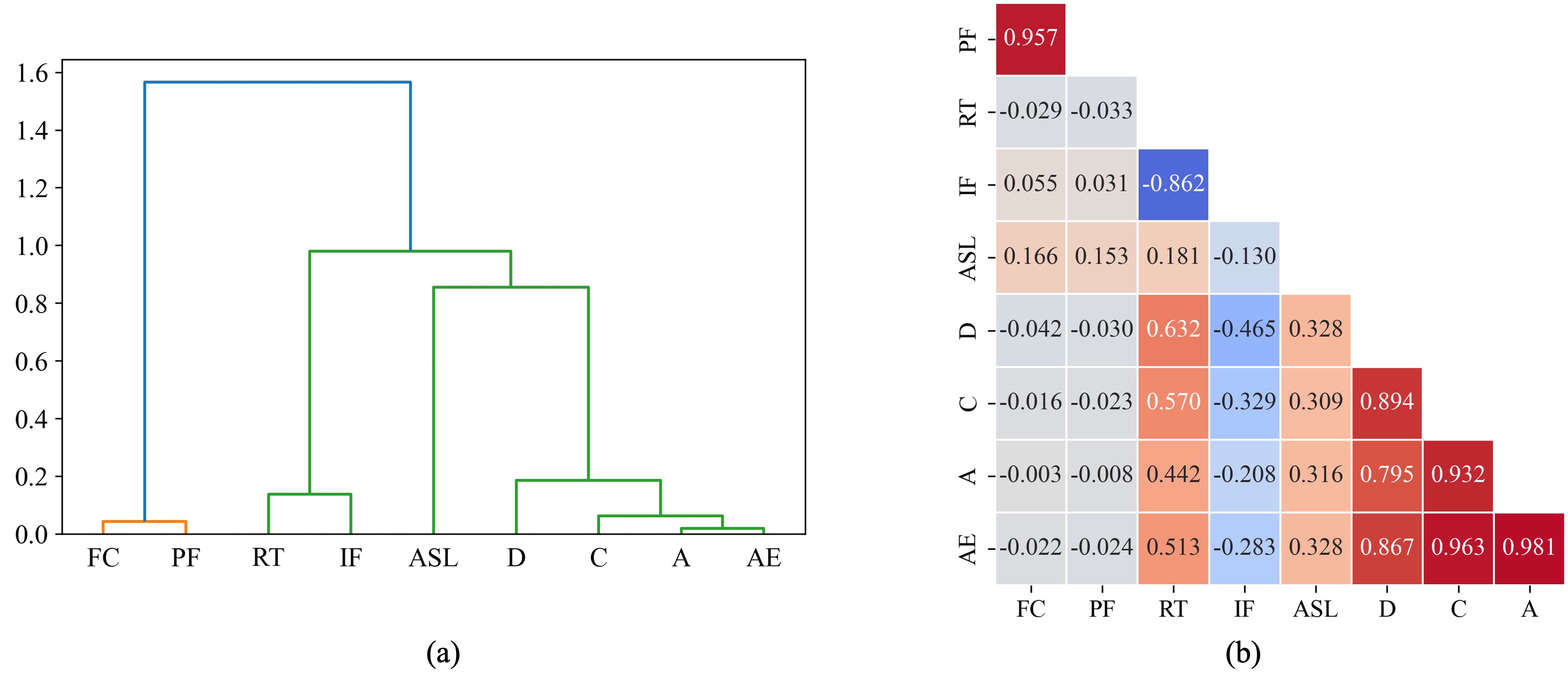
Figure 1:Feature relationship for moisture absorbed composite dataset; (a) hierarchical cluster, (b) Spearman correlation ranking.
As observed in Figure 1a, Frequency Centroid and Peak Frequency are in the same cluster with a highly correlated value of 0.957 shown in Figure 1b. Similarly, Rise Time and Initiation Frequency are clustered with a highly negative correlation of -0.862. Amplitude and Absolute Energy also exhibited a high positive correlation of 0.981.
Table 2 gives the median and interquartile (IQR) feature importance scores based on change in AUC for the LightGBM, RF and SVM models. These scores were obtained using all samples in the PFI process. Values emphasised in bold fonts represent the highest ranked feature for the respective models based on their median change in AUC.
Table 2:Median and IQR feature importance scores based on change in AUC for LightGBM, RF and SVM models, (values in bold fonts represent the highest ranked feature for the respective models).
| Census Income | Bank Marketing | |||||||||||||||||||||
|---|---|---|---|---|---|---|---|---|---|---|---|---|---|---|---|---|---|---|---|---|---|---|
| ID | Feature | LightGBM | RF | SVM | ID | Feature | LightGBM | RF | SVM | |||||||||||||
| Med | IQR | Med | IQR | Med | IQR | Med | IQR | Med | IQR | Med | IQR | |||||||||||
| 25th | 75th | 25th | 75th | 25th | 75th | 25th | 75th | 25th | 75th | 25th | 75th | |||||||||||
| 0 | Age | 0.117 | 0.114 | 0.121 | 0.066 | 0.061 | 0.069 | <10-3 | <10-3 | <10-3 | 0 | Age | 0.016 | 0.015 | 0.017 | 0.026 | 0.024 | 0.027 | -0.001 | -0.001 | 0.002 | |
| 1 | Final weight | -0.002 | -0.003 | -0.001 | <10-3 | -0.003 | 0.004 | 0.003 | <10-3 | 0.011 | 1 | Balance | 0.013 | 0.011 | 0.014 | 0.011 | 0.009 | 0.012 | 0.026 | 0.021 | 0.027 | |
| 2 | Education-num | 0.085 | 0.080 | 0.087 | 0.063 | 0.061 | 0.068 | <10-3 | <10-3 | <10-3 | 2 | Day of week | 0.012 | 0.011 | 0.013 | 0.014 | 0.014 | 0.016 | 0.001 | 0.001> | 0.001 | |
| 3 | Capital-gain | 0.049 | 0.048 | 0.052 | 0.047 | 0.046 | 0.050 | 0.029 | 0.026 | 0.030 | 3 | Duration | 0.256 | 0.253 | 0.261 | 0.211 | 0.209 | 0.215 | 0.154 | 0.148 | 0.157 | |
| 4 | Workclass | <10-3 | <10-3 | 0.001 | 0.003 | 0.001 | 0.004 | <10-3 | <10-3 | <10-3 | 4 | PDays | 0.051 | 0.051 | 0.052 | 0.054 | 0.052 | 0.055 | 0.053 | 0.050 | 0.055 | |
| 5 | Race | <10-3 | <10-3 | <10-3 | 0.001 | 0.001 | 0.002 | <10-3 | <10-3 | <10-3 | 5 | Job_b | 0.003 | 0.003 | 0.004 | 0.002 | 0.001 | 0.002 | <10-3 | <10-3 | <10-3 | |
| 6 | Job_m | <10-3 | <10-3 | 0.001 | 0.001 | 0.001 | 0.002 | <10-3 | <10-3 | <10-3 | ||||||||||||
| 7 | Housing | 0.026 | 0.025 | 0.027 | 0.032 | 0.031 | 0.034 | 0.001 | 0.001 | 0.001 | ||||||||||||
| Statlog (Shuttle) | Diabetes | |||||||||||||||||||||
| 0 | Rad Flow | 0.355 | 0.350 | 0.360 | 0.387 | 0.383 | 0.389 | 0.253 | 0.249 | 0.259 | 0 | HighBP | 0.128 | 0.127 | 0.129 | 0.128 | 0.128 | 0.130 | 0.066 | 0.065 | 0.067 | |
| 1 | Fpv Close | 0.005 | 0.005 | 0.005 | 0.012 | 0.011 | 0.013 | <10-3 | <10-3 | 0.001 | 1 | CholCheck | 0.009 | 0.009 | 0.010 | 0.011 | 0.010 | 0.011 | -0.001 | -0.001 | -0.001 | |
| 2 | Fpv Open | 0.241 | 0.239 | 0.244 | 0.274 | 0.270 | 0.277 | 0.319 | 0.316 | 0.322 | 2 | BMI | 0.080 | 0.078 | 0.081 | 0.079 | 0.077 | 0.080 | -0.073 | -0.074 | -0.072 | |
| 3 | Smoker | 0.004 | 0.004 | 0.005 | 0.004 | 0.004 | 0.005 | 0.026 | 0.025 | 0.027 | ||||||||||||
| Moisture Absorbed Composites | ||||||||||||||||||||||
| 0 | Risetime | 0.005 | 0.005 | 0.005 | 0.009 | 0.008 | 0.009 | 0.004 | 0.003 | 0.004 | ||||||||||||
| 1 | Counts | 0.037 | 0.037 | 0.037 | 0.075 | 0.073 | 0.075 | 0.009 | 0.009 | 0.009 | ||||||||||||
| 2 | ASL | 0.034 | 0.034 | 0.034 | 0.072 | 0.071 | 0.073 | <10-3 | <10-3 | <10-3 | ||||||||||||
| 3 | Freq. Centroid | 0.468 | 0.466 | 0.470 | 0.463 | 0.461 | 0.465 | 0.422 | 0.421 | 0.425 | ||||||||||||
From Table 2, SVM tended to be have very low scores in some datasets, possibly due to its reliance of support vectors in determining the decision boundaries. Thus, features with strong influence at the decision boundary but not directly affecting the support vectors may seem less important. For the Moisture Absorbed Composite dataset, the three classifiers reported similar scores for Frequency Centroid of 0.468, 0.466 and 0.422 respectively in Table 2.
However, in Bank Marketing dataset, LightGBM and RF identified Feature 1 as a relatively important feature, while SVM considered it insignificant. The mutability of importance scores for the classifiers considered underscores the need to explore multiple classifiers when undertaking a comprehensive investigation of feature importance for feature selection purposes.
Figure 2 shows the PFI process time and corresponding sample fractions for the Diabetes dataset, which has a substantial sample size of 253,680 instances. The results are based on one independent run, with PFI set at 30 feature-permuted repeats. For LightGBM and RF, the PFI process time increased linearly with larger sample fractions, whereas SVM experienced an exponential growth. LightGBM had the lowest computational cost, with CPU process times of 3.9 seconds and 28.8 seconds for 10% and 100% sample fractions, respectively. SVM required 21,263 seconds to process the entire dataset, reflecting a 9,345% increase in CPU computational cost compared to using a 10% sample fraction. SVM’s poor performance relative to LightGBM and RF is likely due to its poor CPU parallelisability.
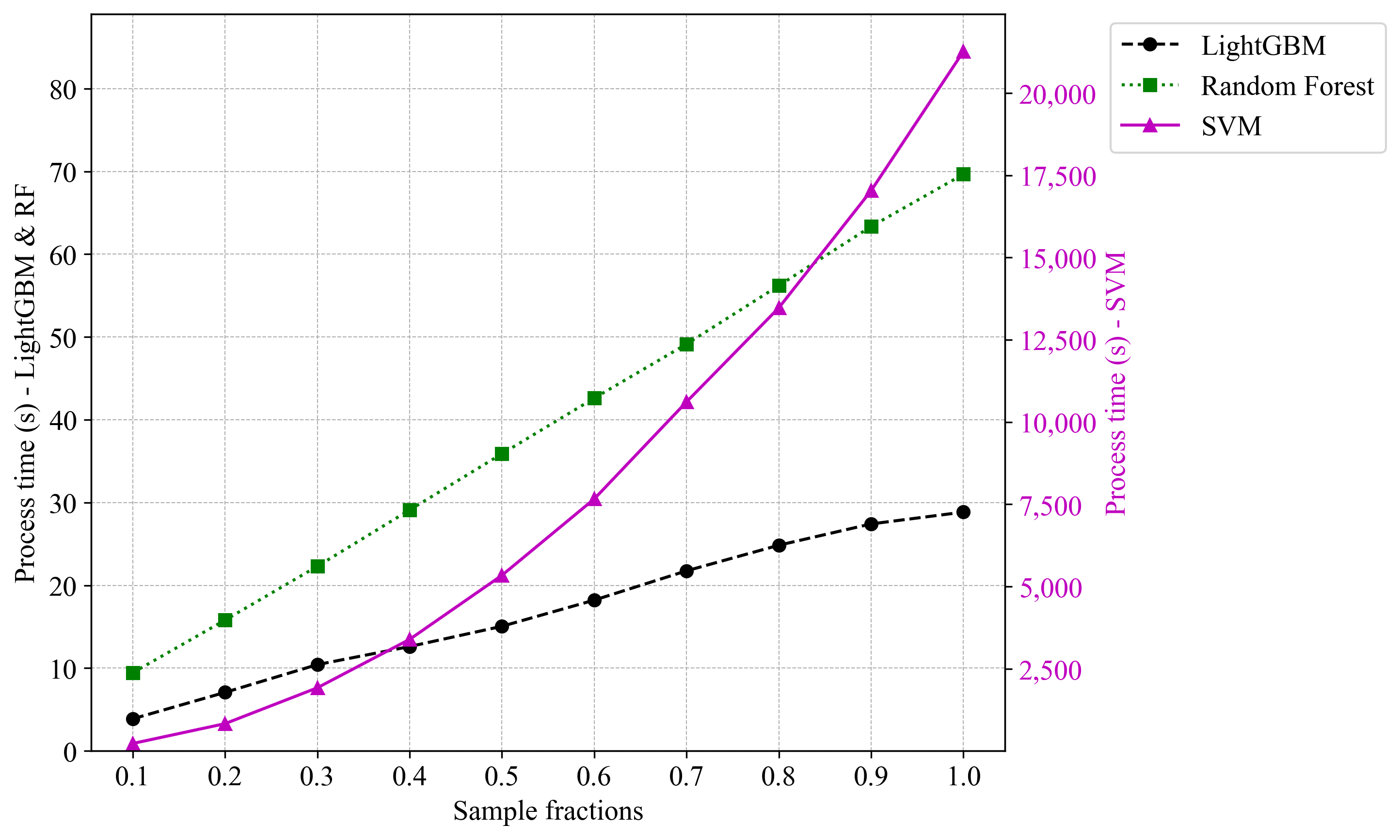
Figure 2:PFI process time and corresponding sample fractions for the Diabetes dataset.
Figure 3a - c present the PFI for Final Weight feature of Census Income dataset, evaluated across different sample fractions using LightGBM, RF, and SVM models, respectively. The change in AUC indicates the impact on model performance when Final Weight feature is permuted. Generally, for smaller sample fractions, there was a higher variability in AUC and prominence of outliers. This could be attributed to the increased influence of randomness, fewer data points, and sampling fluctuations for smaller sample fractions across the datasets.
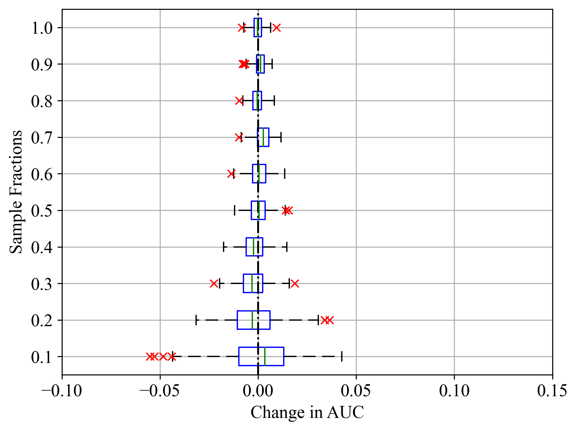
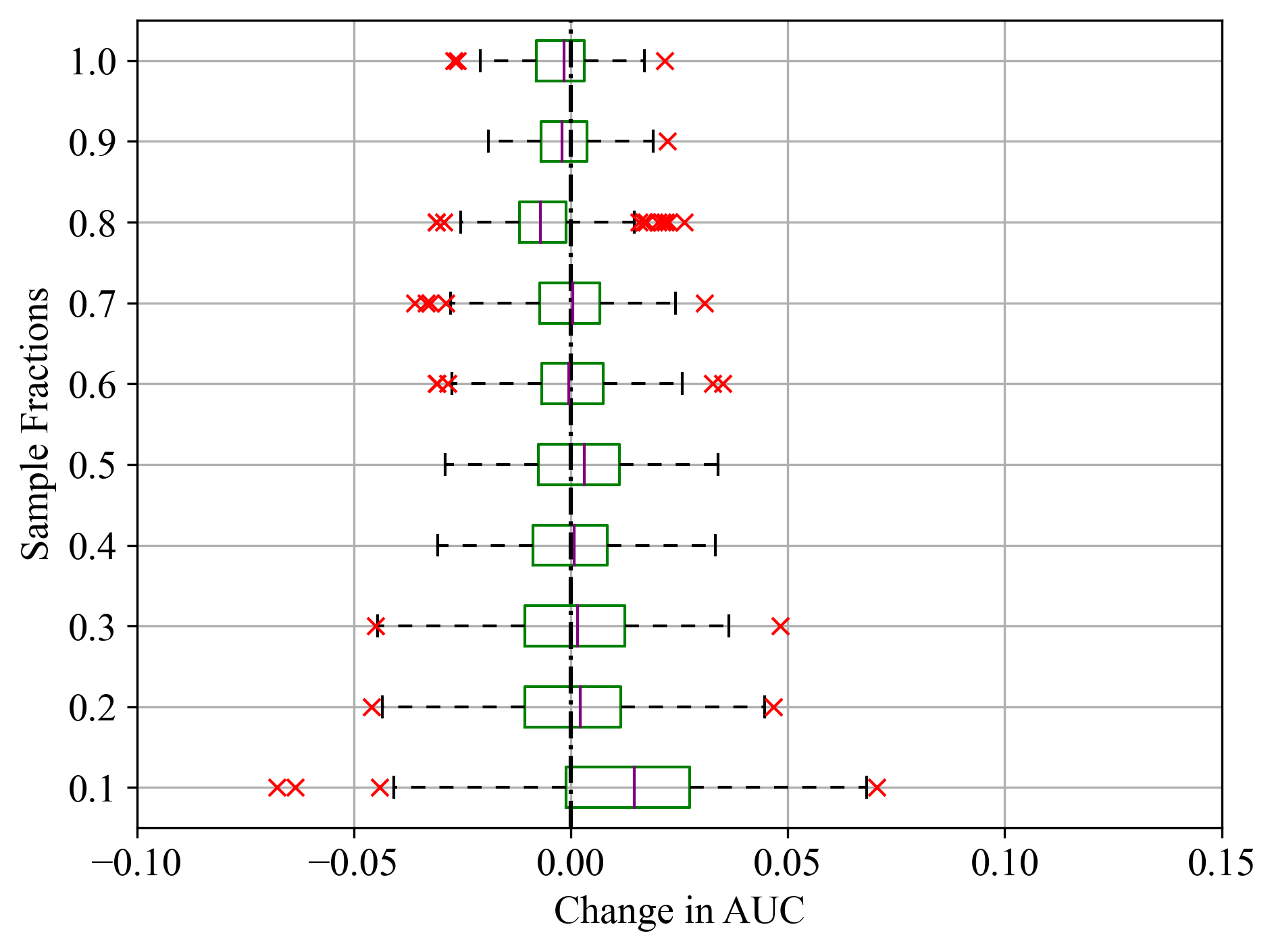
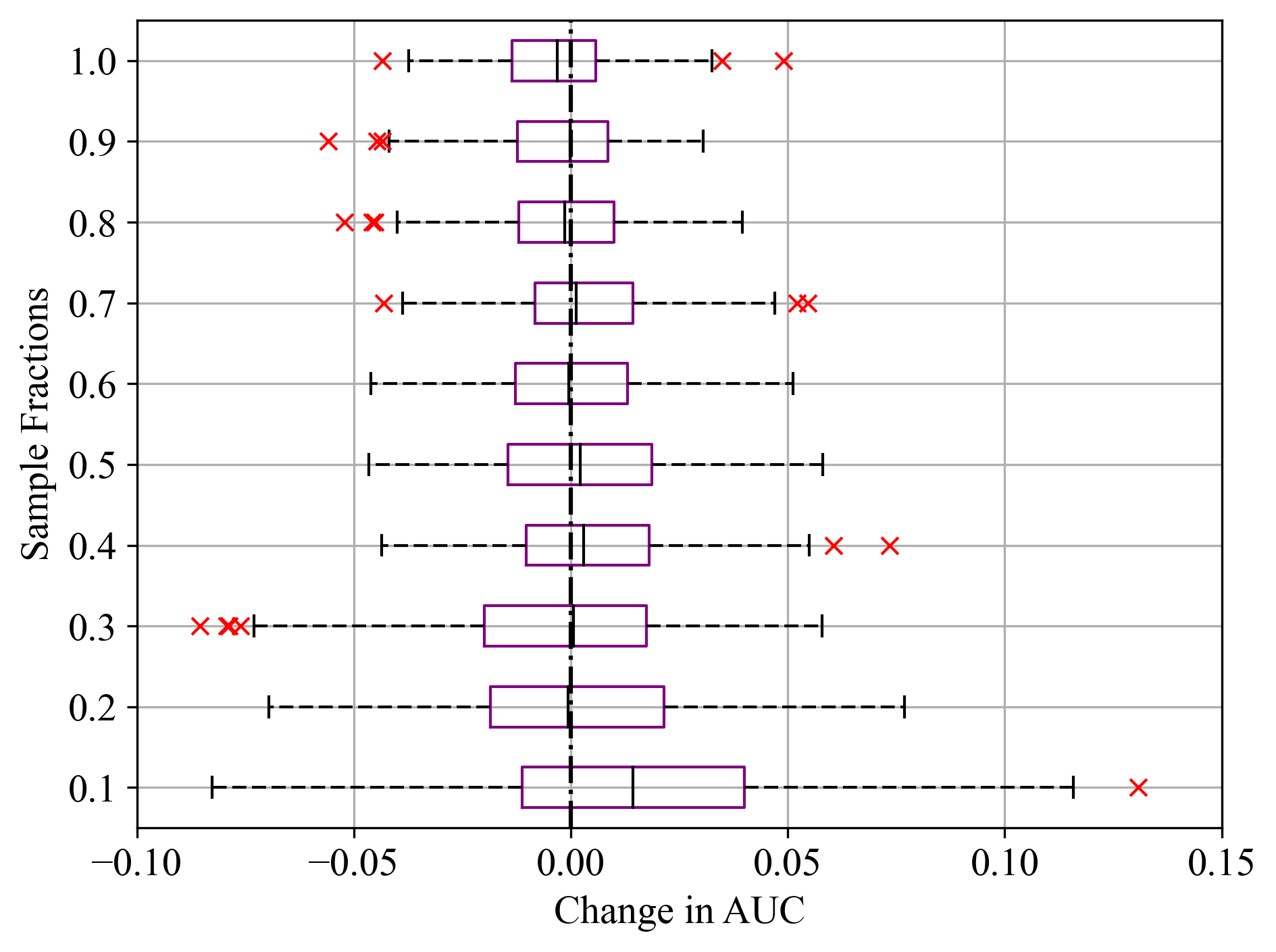
Figure 3:Sample fractions and corresponding change in AUC for Final Weight feature of Census Income dataset; (a) LightGBM, (b) RF, and (c) SVM.
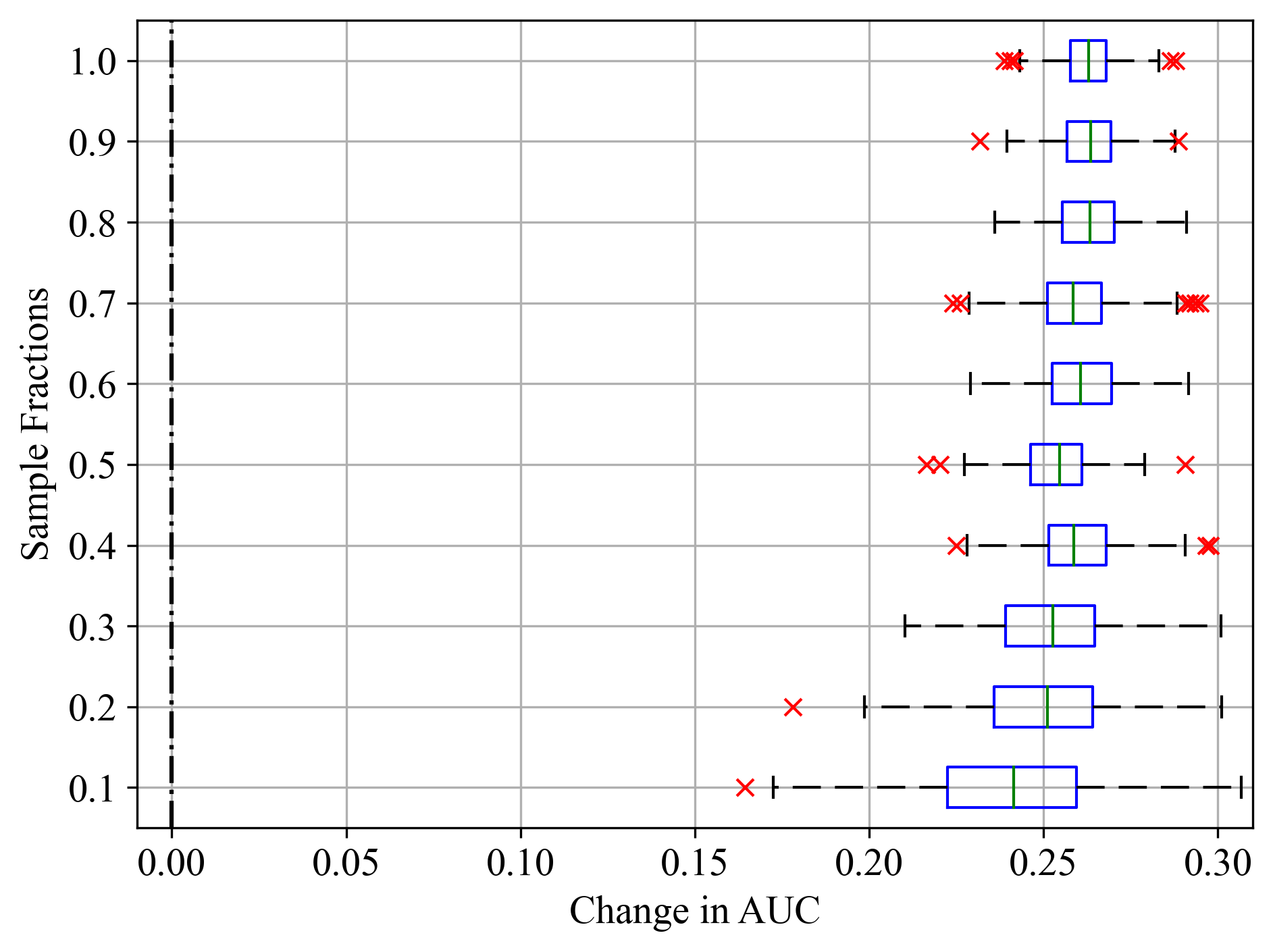
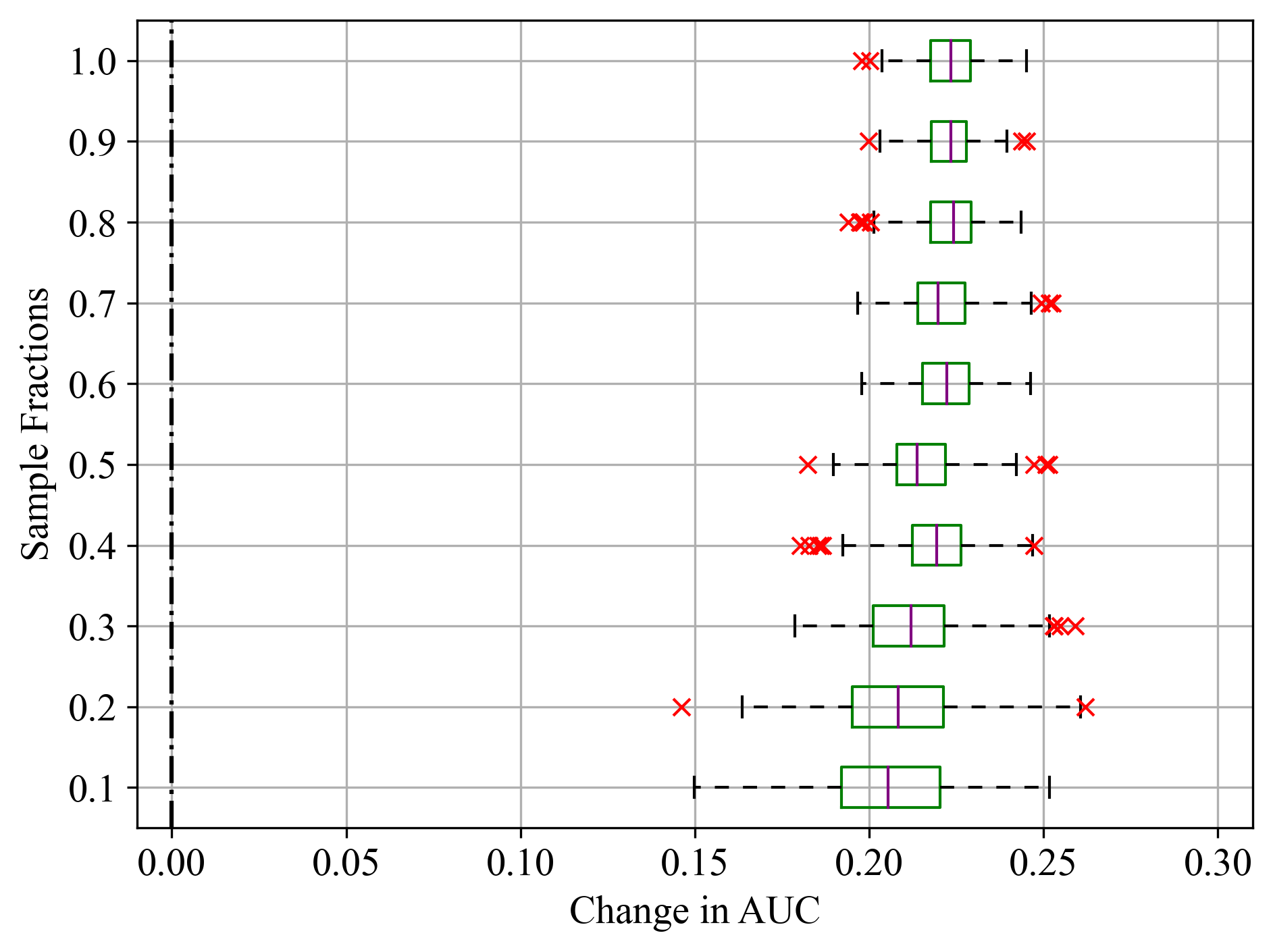
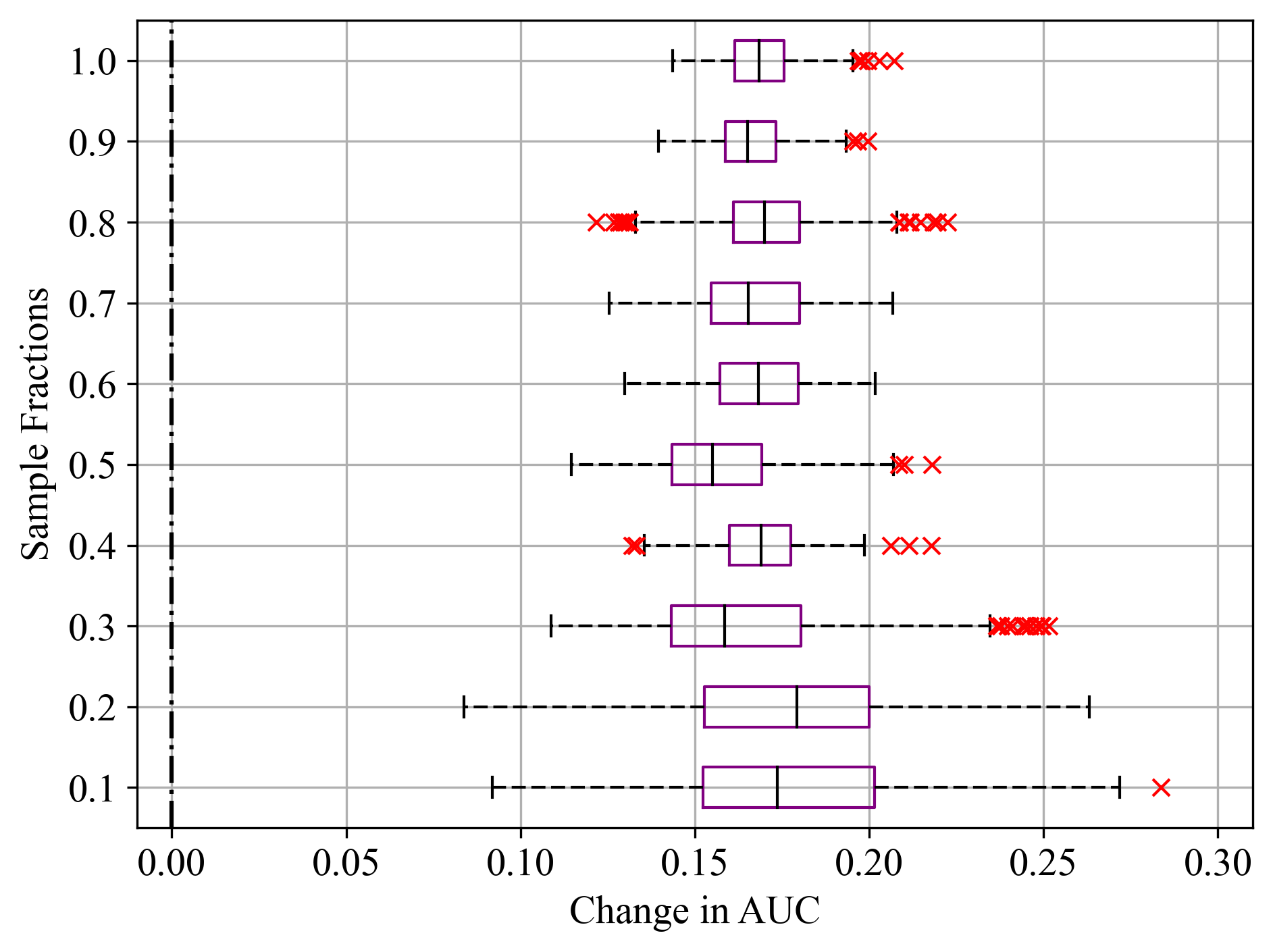
Figure 4:Sample fractions and corresponding change in AUC for Duration feature of Bank Marketing dataset; (a) LightGBM, (b) RF, and (c) SVM.
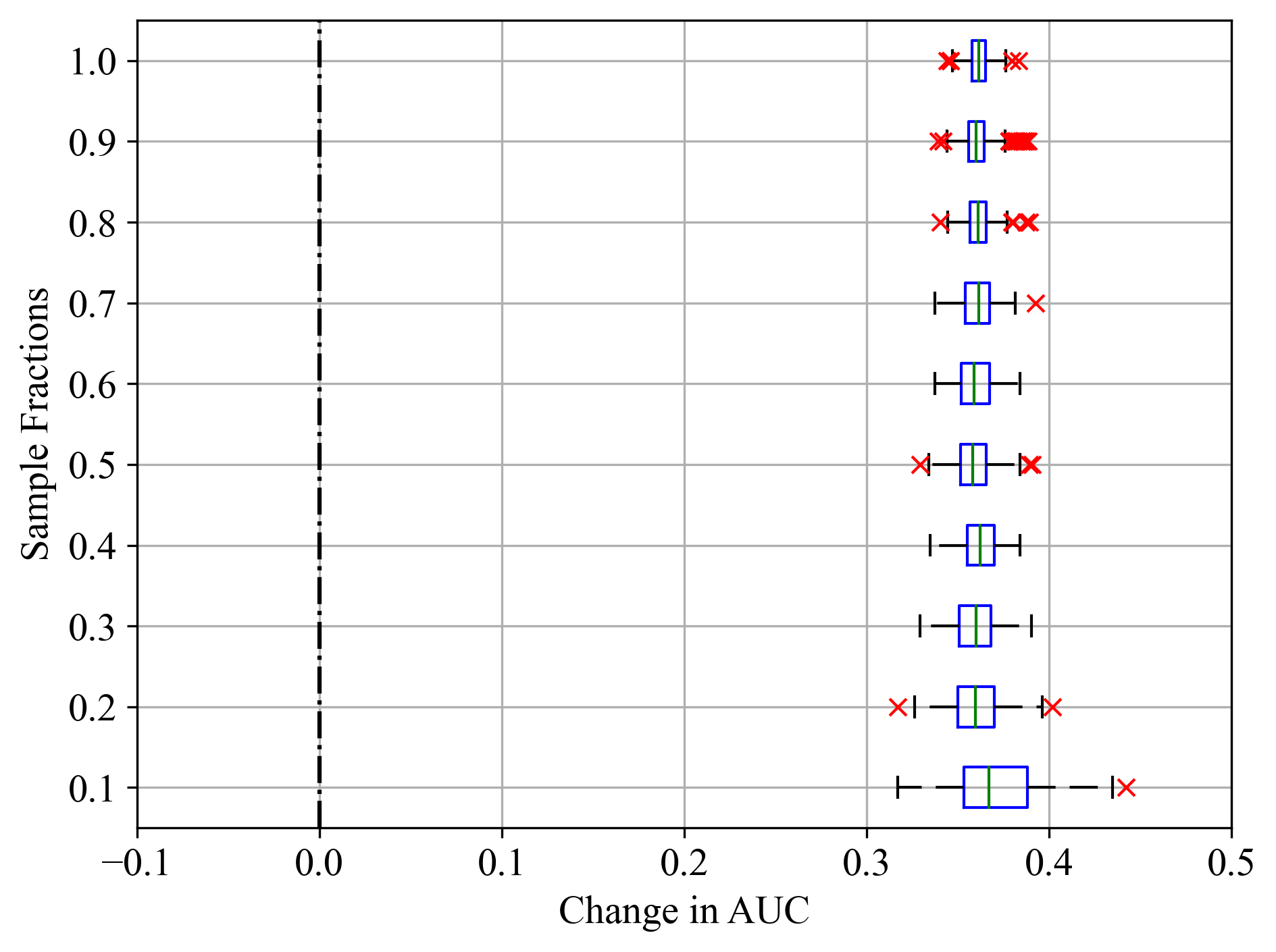
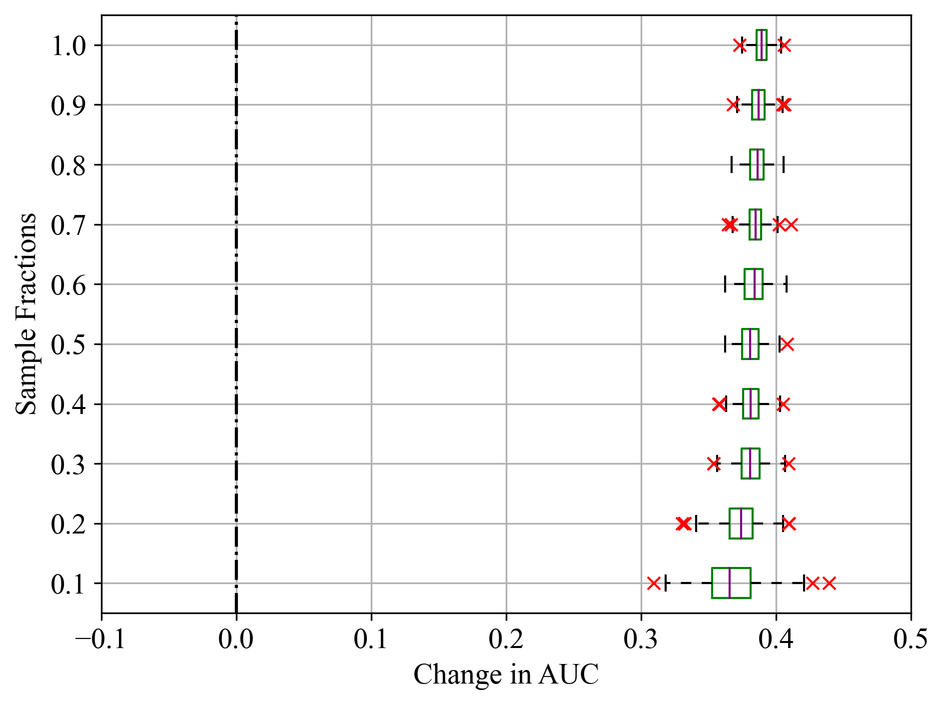
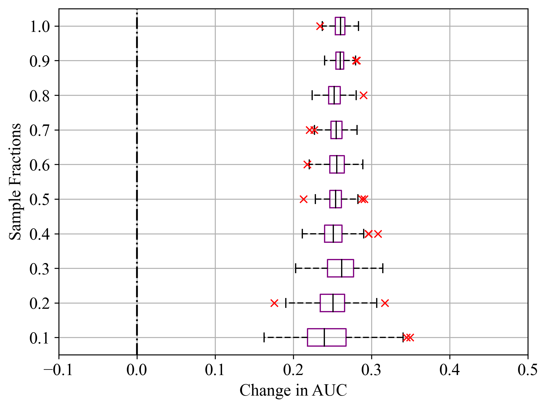
Figure 5:Sample fractions and corresponding change in AUC for Rad Flow feature of Statlog (Shuttle) dataset; (a) LightGBM, (b) RF, and (c) SVM.
For LightGBM model in Figure 3a, the median change in AUC was close to zero, indicating that Final Weight had minimal impact on model performance, as noted in Table 2. Similar results were recorded in Figure 4a - c for the Duration feature of Bank Marketing dataset, where all models exhibited similarly high feature importance scores. Even for sample fractions of 0.5, LightGBM and RF appeared to give similar importance scores to using the entire data sample. On the other hand, SVM exhibited a higher median change in AUC, indicating that the Final Weight feature had a more significant impact on its performance. Additionally, SVM showed the greatest variability and the most prominent outliers, particularly at lower sample fractions. This was noticeable in Figure 5a - c, where all classifiers reported similar importance scores as noted in Table 2. This variability and the presence of outliers suggest that the model’s performance is less stable when features are permuted.
PFI can provide insights into the importance of features, but it is susceptible to variability, especially with smaller sample sizes. Thus, complementary feature selection methods could be explored to validate feature importance. Future work could investigate the variability of features under particular models and sample sizes, with a view to evolving methods of providing a more stable information to the models.
4Conclusion
Feature selection for large datasets incurs considerable computational cost in the model development process of various ML tasks. This study undertakes a preliminary investigation into the influence of sample fractions on feature importance and model performance in datasets characterised by class imbalance. Five real-life datasets with large sample sizes from different subject fields which exhibited high class imbalance ratios of 0.09 – 0.18 were utilised.
Due to its model-agnostic nature, PFI was adopted for feature selection process with feature importance evaluated on Light GBM, RF and SVM. The models were chosen due to their widespread use in real-world ML studies and their role as benchmarks for comparing new models. Cluster, spatial, and stats sub-packages of SciPy were instrumental in tackling the multicollinearity effects associated with PFI. Using a PFI approach, the study revealed the variability of feature importance with smaller sample fractions in LightGBM, random forest and SVM models. In the cases explored, LightGBM showed the lowest variability, while SVM exhibited the highest variability in feature importance. Also, Light GBM had the least CPU process time across the cases considered, while SVM showed the highest computational cost.
In future work, this investigation would be expanded to substantially larger datasets and introduce some quantitative measure of the variability of various models and feature selection methods. An understanding of the variability of feature importance can inform feature engineering efforts that provides means of alleviating the variability of feature importance in samples fractions under class imbalance conditions.
This work was supported by the Petroleum Technology Development Fund under grant PTDF/ED/OSS/PHD/AGU/1076/17 and NISCO UK Research Centre. Computations were performed using the Sulis Tier 2 HPC platform hosted by the Scientific Computing Research Technology Platform at the University of Warwick. Sulis is funded by EPSRC Grant EP/T022108/1 and the HPC Midlands+ consortium.
Copyright © 2024 Udu et al. This is an open-access article distributed under the terms of the Creative Commons Attribution 4.0 International license, which enables reusers to distribute, remix, adapt, and build upon the material in any medium or format, so long as attribution is given to the creators.
- AUC
- area under the Receiver Operator Characteristics (ROC) curve
- IQR
- Interquartile range
- Light GBM
- Light Gradient-Boosting Machine
- ML
- machine learning
- PFI
- Permutation Feature Importance
- RF
- Random Forest
- ROC
- Receiver Operator Characteristics
- SVM
- Support Vector Machines
- Cai, J., Luo, J., Wang, S., & Yang, S. (2018). Feature selection in machine learning: A new perspective. Neurocomputing, 300, 70–79. 10.1016/j.neucom.2017.11.077
- Dhal, P., & Azad, C. (2022). A comprehensive survey on feature selection in the various fields of machine learning. Applied Intelligence. 10.1007/s10489-021-02550-9
- Udu, A. G., Lecchini-Visintini, A., & Dong, H. (2023). Feature Selection for Aero-Engine Fault Detection (Vol. 3). Springer Nature. 10.1007/978-3-031-39847-6_42
- Yin, L., Ge, Y., Xiao, K., Wang, X., & Quan, X. (2013). Feature selection for high-dimensional imbalanced data. Neurocomputing, 105, 3–11. 10.1016/j.neucom.2012.04.039
- Tsai, C.-F., & Sung, Y.-T. (2020). Ensemble feature selection in high dimension, low sample size datasets: Parallel and serial combination approaches. Knowledge-Based Systems, 203, 106097. 10.1016/j.knosys.2020.106097
- de Haro-García, A., Cerruela-García, G., & García-Pedrajas, N. (2020). Ensembles of feature selectors for dealing with class-imbalanced datasets: A proposal and comparative study. Information Sciences, 540, 89–116. 10.1016/j.ins.2020.05.077
- Matharaarachchi, S., Domaratzki, M., & Muthukumarana, S. (2021). Assessing feature selection method performance with class imbalance data. Machine Learning with Applications, 6, 100170. 10.1016/j.mlwa.2021.100170
- Bonaccorso, G. (2018). Machine Learning Algorithms: Popular algorithms for data science and machine learning. Packt Publishing Ltd.
- Feng, S., Zhou, H., & Dong, H. (2019). Using deep neural network with small dataset to predict material defects. Materials & Design, 162, 300–310. 10.1177/07316844241236696
- Sarker, I. H. (2021). Machine learning: Algorithms, real-world applications and research directions. SN Computer Science, 2(3), 160. 10.1007/s42979-021-00592-x
- Paleyes, A., Urma, R.-G., & Lawrence, N. D. (2022). Challenges in deploying machine learning: a survey of case studies. ACM Computing Surveys, 55(6), 1–29. 10.1145/3533378
- Udu, A. G., Osa-uwagboe, N., Adeniran, O., Aremu, A., Khaksar, M. G., & Dong, H. (2024). A machine learning approach to characterise fabrication porosity effects on the mechanical properties of additively manufactured thermoplastic composites. Journal of Reinforced Plastics and Composites, 07316844241236696. 10.1177/07316844241236696
- Luque, A., Carrasco, A., Martín, A., & de las Heras, A. (2019). The impact of class imbalance in classification performance metrics based on the binary confusion matrix. Pattern Recognition, 91, 216–231. 10.1016/j.patcog.2019.02.023
- Temraz, M., & Keane, M. T. (2022). Solving the class imbalance problem using a counterfactual method for data augmentation. Machine Learning with Applications, 9, 100375. 10.1016/j.mlwa.2022.100375
- The Pandas Development Team. (2020). pandas-dev/pandas: Pandas (latest). Zenodo. 10.5281/zenodo.3509134
