
Using Blosc2 NDim As A Fast Explorer Of The Milky Way (Or Any Other NDim Dataset)
Abstract
Large multidimensional datasets are widely used in various engineering and scientific applications. Prompt access to the subsets of these datasets is crucial for an efficient exploration experience. To facilitate this, we have added support for large dimensional datasets to Blosc2, a compression and format library. The extension enables effective support for large multidimensional datasets, with a special encoding of zeros that allows for efficient handling of sparse datasets. Additionally, the new two-level data partition used in Blosc2 reduces the need for decompressing unnecessary data, further accelerating slicing speed.
The Blosc2 NDim layer enables the creation and reading of n-dimensional datasets in an extremely efficient manner. This is due to a completely general n-dim 2-level partitioning, which allows for slicing and dicing of arbitrary large (and compressed) data in a more fine-grained way. Having a second partition provides a better flexibility to fit the different partitions at the different CPU cache levels, making compression even more efficient.
Additionally, Blosc2 can make use of Btune, a library that automatically finds the optimal combination of compression parameters to suit user needs. Btune employs various techniques, such as a genetic algorithm and a neural network model, to discover the best parameters for a given dataset much more quickly. This approach is a significant improvement over the traditional trial-and-error method, which can take hours or even days to find the best parameters.
As an example, we will demonstrate how Blosc2 NDim enables fast exploration of the Milky Way using the Gaia DR3 dataset.
Introduction
The exploration of datasets that are high dimensional is a common practice in various fields of science. However, exploring such n-dimensional datasets is challenging when the memory size of the dataset is extremely large. This can slow down the data exploration process significantly. In this paper, we demonstrate how Blosc2 NDim can be used to accelerate the exploration of huge n-dimensional datasets.
Blosc is a high-performance compressor optimized for binary data. Its design enables faster transmission of data to the processor cache than the traditional, non-compressed, direct memory fetch approach using an OS call to memcpy(). This can be helpful not only in reducing the size of large datasets on-disk and in-memory, but also in accelerating memory-bound computations, which are typical in big data processing.
Blosc uses the blocking technique Francesc Alted (2010) to minimize activity on the memory bus. The technique divides datasets into blocks small enough to fit in the caches of modern processors, where compression/decompression is performed. Blosc also takes advantage of single-instruction multiple-data streams (SIMD), like SSE2, AVX2, NEON… and multi-threading capabilities in modern multi-core processors to maximize the compression/decompression speed.
In addition, using the Blosc compressed data can accelerate memory-bound computations when enough cores are dedicated to the task. Figure 1 provides a real example of this.
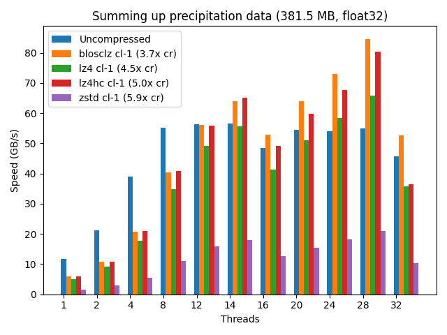
Figure 1:Speed for summing up a vector of real float32 data (meteorological precipitation) using a variety of codecs provided by Blosc2. Note that the maximum speed is achieved when utilizing the maximum number of (logical) threads available on the computer (28), where different codecs are allowing faster computation than using uncompressed data. Benchmark performed on a Intel i9-10940X CPU, with 14 physical cores. More info at Francesc Alted (2018).
Blosc2 is the latest version of the Blosc 1.x series, which is used in many important libraries, such as HDF5 The HDF Group (1997), Zarr Zarr Developers (2017), and PyTables PyTables developers (2002). Its NDim feature excels at reading multi-dimensional slices, thanks to an innovative pineapple-style partitioning technique Francesc Alted and Oscar Guiñón (2023). This enables fast exploration of general n-dimensional datasets, including the 3D Gaia array.
The Milky Way dataset
Figure 2 shows a 3D view of the Milky Way different type of stars. Each point is a star, and the color of each point represents the star’s magnitude, with the brightest stars appearing as the reddest points. Although this view provides a unique perspective, the dimensions of the cube are not enough to fully capture the spiral arms of the Milky Way.
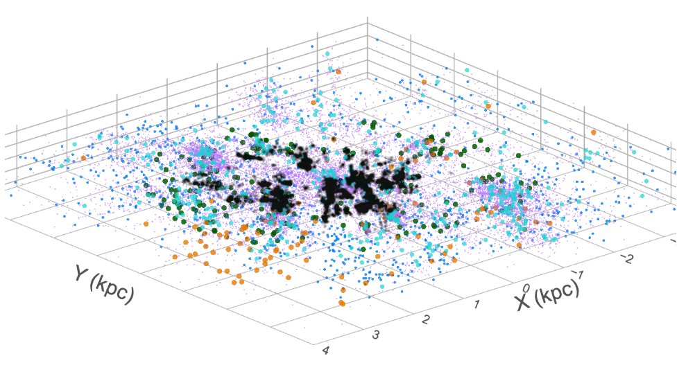
Figure 2:Gaia DR3 dataset as a 3D array (Gaia collaboration).
One advantage of using a 3D array is the ability to utilize Blosc2 NDim’s powerful slicing capabilities for quickly exploring parts of the dataset. For example, we could search for star clusters by extracting small cubes as NumPy arrays, and counting the number of stars in each one. A cube containing an abnormally high number of stars would be a candidate for a cluster. We could also extract a thin 3D slice of the cube and project it as a 2D image, where the pixels colors represent the magnitude of the shown stars. This could be used to generate a cinematic view of a journey over different trajectories in the Milky Way.
For getting the coordinates of the stars in the Milky Way, we will be using the Gaia DR3 dataset European Space Agency (ESA) and Gaia Data Processing and Analysis Consortium (DPAC) (2023), a catalog containing information on 1.7 billion stars in our galaxy. For this work, we extracted the 3D coordinates of 1.4 billion stars (those with non-null parallax values). When stored as a binary table, the dataset is 22 GB in size (uncompressed).
We converted the tabular dataset into a sphere with a radius of 10,000 light years and framed it into a 3D array of shape (20,000, 20,000, 20,000). Each cell in the array represents a cube of 1 light year per side and contains the number of stars within it. Given that the average distance between stars in the Milky Way is about 5 light years, very few cells will contain more than one star (e.g. the maximum of stars in a single cell in our sphere is 6). This 3D array contains 0.5 billion stars, which is a significant portion of the Gaia catalog.
The number of stars is stored as a uint8, resulting in a total dataset size of 7.3 TB. However, compression can greatly reduce its size to 2.2 GB since the 3D array is very sparse, and the Zstandard codec zstd is used. Blosc2 can compress the zeroed parts almost entirely thanks to a specific algorithm to detect zeros early in the compression pipeline and encoding them efficiently.
In addition, we store other data about the stars in a separate table indexed with the position of each star (using PyTables). For demonstration purposes, we store the distance from Sun, radial velocity, effective temperature, and G-band magnitude using a float32 for each field. The size of the table is 10 GB uncompressed, but it can be compressed to 4.8 GB. Adding another 1.0 GB for the index brings the total size to 5.8 GB. Therefore, the 3D array is 2.2 GB, and the table with the additional information and its index are 5.8 GB, making a total of 8.0 GB. This comfortably fits within the storage capacity of any modern laptop.
Blosc2 NDim
In the plain Blosc and Blosc2 libraries, there are two levels of partitioning: the block and the chunk. The block is the smallest unit of data that can be compressed and decompressed independently. The chunk is a group of blocks that are compressed together. The chunk and block sizes are parameters that can be tuned to fit the different cache levels in modern CPUs. For optimal performance, it is recommended that the block size should fit in the L1 or L2 CPU cache, minimizing contention between worker threads during compression/decompression. The chunk size, on the other hand, should fit in the L3 CPU cache, in order to minimize data movement to RAM and speed up decompression.
With Blosc2 NDim, we are taking this feature a step further and both partitions, known as chunks and blocks, are gaining multidimensional capabilities. This means that one can split a dataset (called a “super-chunk” in Blosc2 terminology) into n-dimensional cubes and sub-cubes. Refer to Figures Figure 3 and Figure 4 to learn more about how this works and how to set it up.
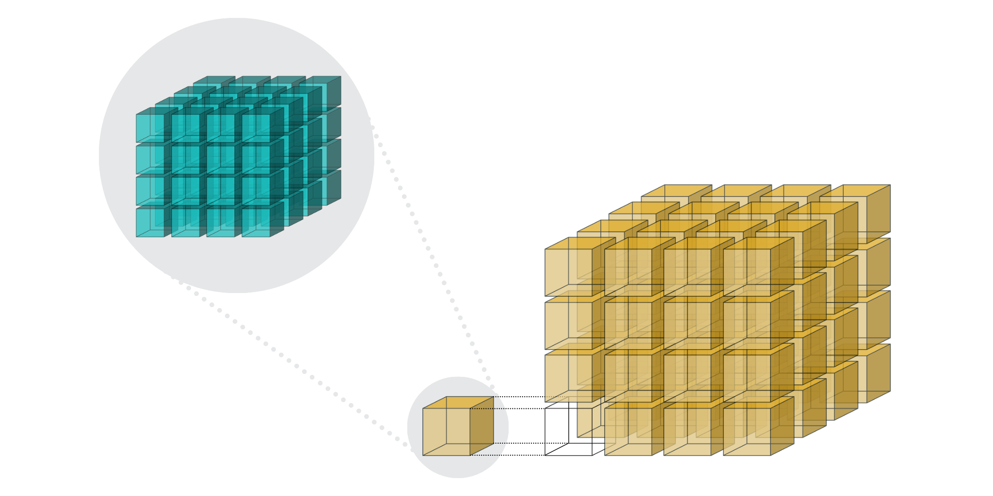
Figure 3:Blosc2 NDim 2-level partitioning.
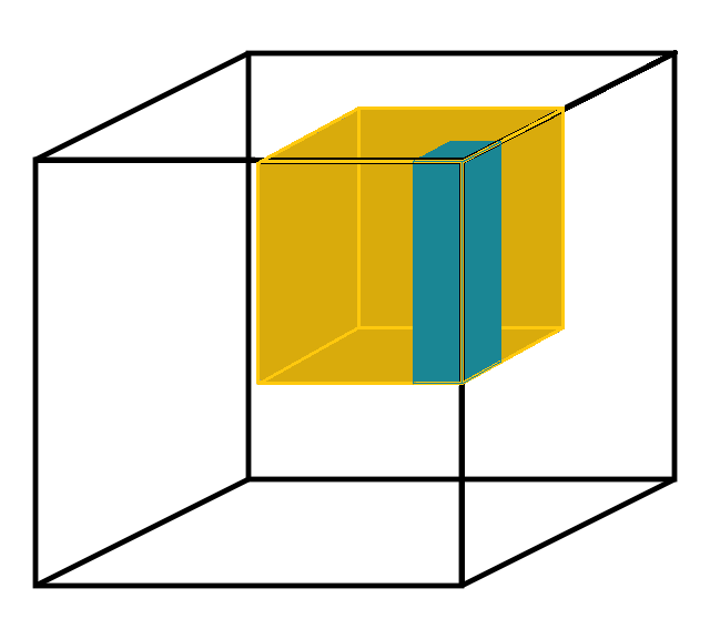
Figure 4:Blosc2 NDim 2-level partitioning is flexible. The dimensions of both partitions can be specified in any arbitrary way that fits the expected read access patterns.
With these finer-grained cubes, arbitrary n-dimensional slices can be retrieved faster. This is because not all the data necessary for the coarser-grained partition has to be decompressed, as is typically required in other libraries (see Figure 5).
For example, for a 4-d array with a shape of (50, 100, 300, 250) with float64 items, we can choose a chunk with shape (10, 25, 50, 50) and a block with shape (3, 5, 10, 20) which makes for about 5 MB and 23 KB respectively. This way, a chunk fits comfortably on a L3 cache in most of modern CPUs, and a block in a L1 cache (we are tuning for speed here). See Figure 6 for a speed comparison with other libraries supporting just one single n-dimensional partition.
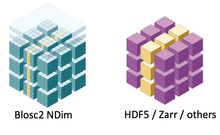
Figure 5:Blosc2 NDim can decompress data faster by using double partitioning, which allows for higher data selectivity. This means that less data compression/decompression is required in general.
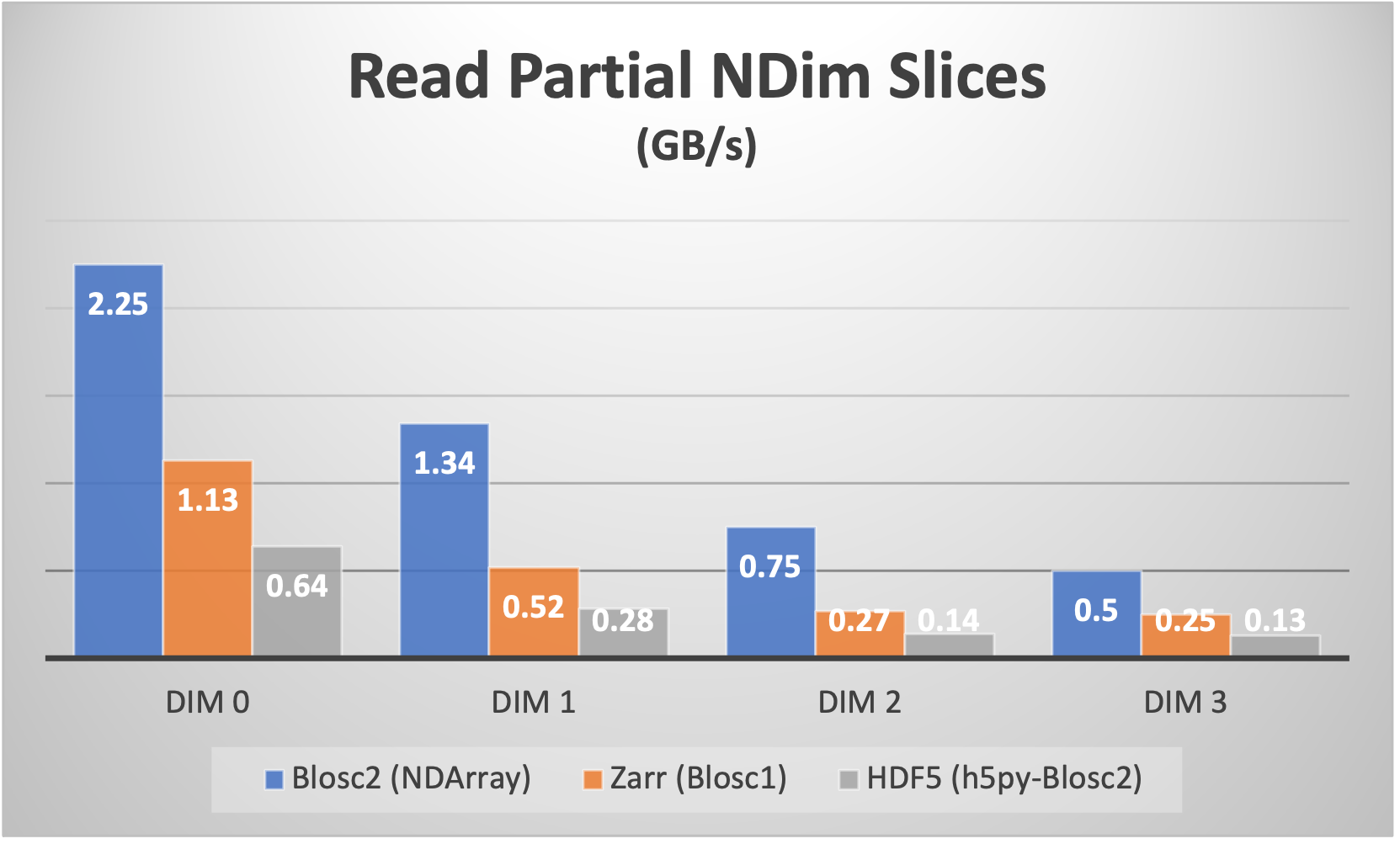
Figure 6:Speed comparison for reading partial n-dimensional slices of a 4D dataset. The legends labeled “DIM N” refer to slices taken orthogonally to each dimension. The sizes for the two partitions have been chosen such that the first partition fits comfortably in the L3 cache of the CPU (Intel i9 13900K), and the second partition fits in the L1 cache of the CPU. Francesc Alted and Oscar Guiñón (2023).
Finally, Blosc2 NDim supports all data types in NumPy. This means that, in addition to the typical data types like signed/unsigned int, single and double-precision floats, bools or strings, it can also store datetimes (including units), and arbitrarily nested heterogeneous types. This allows to create multidimensional tables and more.
Support for multiple codecs, filters, and other compression features
Blosc2 is not only a compression library, but also a framework for creating efficient compression pipelines. A compression pipeline is composed of a sequence of filters, followed by a compression codec. A filter is a transformation that is applied to the data before compression, and a codec is a compression algorithm that is applied to the filtered data. Filters can lead to better compression ratios and improved compression/decompression speeds.
Blosc2 supports a variety of codecs, filters, and other compression features. In particular, it supports the following codecs out-of-the-box:
- BloscLZ (fast codec, the default),
- LZ4 (a very fast codec),
- LZ4HC (high compression variant of LZ4),
- Zlib (the Zlib-NG variant of Zlib),
- Zstd (high compression), and
- ZFP (lossy compression for n-dimensional datasets of floats).
It also supports the following filters out-of-the-box:
- Shuffle (groups equal significant bytes together, useful for ints/floats),
- Shuffle with bytedelta (same than shuffle, but storing deltas of consecutive same significant bytes),
- Bitshuffle (groups equal significant bits together, useful for ints/floats), and
- Truncation (truncates precision, useful for floats; lossy).
Blosc2 utilizes a pipeline architecture that enables the chaining of different filters Marta Iborra (2022) followed by a compression codec. Additionally, it allows for pre-filters (user code meant to be executed before the pipeline) and post-filters (user code meant to be executed after the pipeline). This architecture is highly flexible and minimizes data copies between the different steps, making it possible to create highly efficient pipelines for a variety of use cases. Figure 7 illustrates how this works.
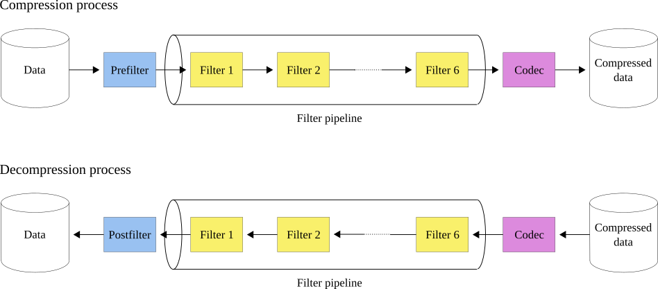
Figure 7:The Blosc2 filter pipeline. During compression, the first function applied is the prefilter (if any), followed by the filter pipeline (with a maximum of six filters), and finally, the codec. During decompression, the order is reversed: first the codec, then the filter pipeline, and finally the postfilter (if any).
Furthermore, Blosc2 supports user-defined codecs and filters, allowing one to create their own compression algorithms and use them within Blosc2 Marta Iborra (2022). These user-defined codecs and filters can also be dynamically loaded Marta Iborra and Francesc Alted (2023), registered globally within Blosc2, and installed via a Python wheel so that they can be used seamlessly from any Blosc2 application (whether in C, Python, or any other language that provides a Blosc2 wrapper).
Automatic tuning of compression parameters
Finding the right compression parameters for the data is probably the most difficult part of using a compression library. Which combination of code and filters would provide the best compression ratio? Which one would provide the best compression/decompression speed?
Btune is an AI tool for Blosc2 that automatically finds the optimal combination of compression parameters to suit user needs. It uses a neural network trained on representative datasets to be compressed to predict the best compression parameters based on the given tradeoff between compression ratio and compression/decompression speed.
For example, Table 1 displays the results for the predicted compression parameters tuned for decompression speed of the 3D Gaia array. This table can be provided to the Btune plugin so that it can choose the best tradeoff value for user’s needs (0 means favoring speed only, and 1 means favoring compression ratio only).
Table 1:Btune prediction of the best compression parameters for decompression speed for the 3D Gaia array, depending on a tradeoff value between compression ratio and decompression speed. It can be seen that BloscLZ with compression level 5 is the most predicted category when decompression speed is preferred, whereas Zstd with compression level 9 + BitShuffle is the most predicted one when the specified tradeoff is towards optimizing for the compression ratio. Speeds are in GB/s.
| Tradeoff | Most predicted | Cratio | Cspeed | Dspeed |
|---|---|---|---|---|
| 0.0 | blosclz-nofilter-5 | 786.51 | 106.86 | 91.04 |
| 0.1 | blosclz-nofilter-5 | 786.51 | 106.86 | 91.04 |
| 0.2 | blosclz-nofilter-5 | 786.51 | 106.86 | 91.04 |
| 0.3 | blosclz-nofilter-5 | 786.51 | 106.86 | 91.04 |
| 0.4 | blosclz-nofilter-5 | 786.51 | 106.86 | 91.04 |
| 0.5 | blosclz-nofilter-5 | 786.51 | 106.86 | 91.04 |
| 0.6 | zstd-nofilter-9 | 8959.6 | 8.79 | 59.13 |
| 0.7 | zstd-nofilter-9 | 8959.6 | 8.79 | 59.13 |
| 0.8 | zstd-nofilter-9 | 8959.6 | 8.79 | 59.13 |
| 0.9 | zstd-bitshuffle-9 | 10789.6 | 3.41 | 12.78 |
| 1.0 | zstd-bitshuffle-9 | 10789.6 | 3.41 | 12.78 |
Of course, results will be different for another dataset. For example, Table 2 displays the results for the predicted compression parameters tuned for decompression speed for a dataset coming from cancer imaging. Curiously, in this case fast decompression does not necessarily imply fast compression.
Table 2:Btune prediction of the best compression parameters for decompression speed for another dataset (cancer imaging). It can be seen that BloscLZ with compression level 5 + Shuffle is the most predicted category when decompression speed is preferred, whereas Zstd (either compression level 1 or 9) + Shuffle + ByteDelta is the most predicted one when the specified tradeoff is towards optimizing for the compression ratio. Speeds are in GB/s.
| Tradeoff | Most predicted | Cratio | Cspeed | Dspeed |
|---|---|---|---|---|
| 0.0 | blosclz-shuffle-5 | 2.09 | 14.47 | 48.93 |
| 0.1 | blosclz-shuffle-5 | 2.09 | 14.47 | 48.93 |
| 0.2 | blosclz-shuffle-5 | 2.09 | 14.47 | 48.93 |
| 0.3 | blosclz-shuffle-5 | 2.09 | 14.47 | 48.93 |
| 0.4 | zstd-bytedelta-1 | 3.30 | 17.04 | 21.65 |
| 0.5 | zstd-bytedelta-1 | 3.30 | 17.04 | 21.65 |
| 0.6 | zstd-bytedelta-1 | 3.30 | 17.04 | 21.65 |
| 0.7 | zstd-bytedelta-1 | 3.30 | 17.04 | 21.65 |
| 0.8 | zstd-bytedelta-1 | 3.30 | 17.04 | 21.65 |
| 0.9 | zstd-bytedelta-1 | 3.30 | 17.04 | 21.65 |
| 1.0 | zstd-bytedelta-9 | 3.31 | 0.07 | 11.40 |
On the other hand, there are also situations where data have to be compressed at a high speed (e.g. consolidating data from high bandwidth detectors). Table 3 shows an example of predicted compression parameter tuned this time for compression speed and ratio on yet another dataset for this scenario (in this case, images coming from synchrotron facilities).
Table 3:Btune prediction of the best compression parameters for compression speed (synchrotron imaging). It can be seen that LZ4 with compression level 5 + Bitshuffle is the most predicted category when compression speed is preferred, whereas Zstd (either compression level 1 or 9) + Shuffle + ByteDelta is the most predicted one when the specified tradeoff is leveraged towards the compression ratio. Speeds are in GB/s.
| Tradeoff | Most predicted | Cratio | Cspeed | Dspeed |
|---|---|---|---|---|
| 0.0 | lz4-bitshuffle-5 | 3.41 | 21.78 | 32.0 |
| 0.1 | lz4-bitshuffle-5 | 3.41 | 21.78 | 32.0 |
| 0.2 | lz4-bitshuffle-5 | 3.41 | 21.78 | 32.0 |
| 0.3 | lz4-bitshuffle-5 | 3.41 | 21.78 | 32.0 |
| 0.4 | lz4-bitshuffle-5 | 3.41 | 21.78 | 32.0 |
| 0.5 | lz4-bitshuffle-5 | 3.41 | 21.78 | 32.0 |
| 0.6 | lz4-bitshuffle-5 | 3.41 | 21.78 | 32.0 |
| 0.7 | lz4-bitshuffle-5 | 3.41 | 21.78 | 32.0 |
| 0.8 | zstd-bytedelta-1 | 3.98 | 9.41 | 18.8 |
| 0.9 | zstd-bytedelta-1 | 3.98 | 9.41 | 18.8 |
| 1.0 | zstd-bytedelta-9 | 4.06 | 0.15 | 14.1 |
After training the neural network, the Btune plugin can automatically tune the compression parameters for a given dataset. During inference, the user can set the preferred tradeoff by setting the BTUNE_TRADEOFF environment variable to a floating point value between 0 and 1. A value of 0 favors speed only, while a value of 1 favors compression ratio only. This setting automatically selects the compression parameters most suitable to the current data chunk whenever a new Blosc2 data container is being created.
Results on the Gaia dataset
We will use the training results above to compress the big 3D Gaia array so that it can be explored more quickly. Figure 8 displays the speed that can be achieved when getting multiple multidimensional slices of the dataset along different axes, using the most efficient codecs and filters for various tradeoffs.
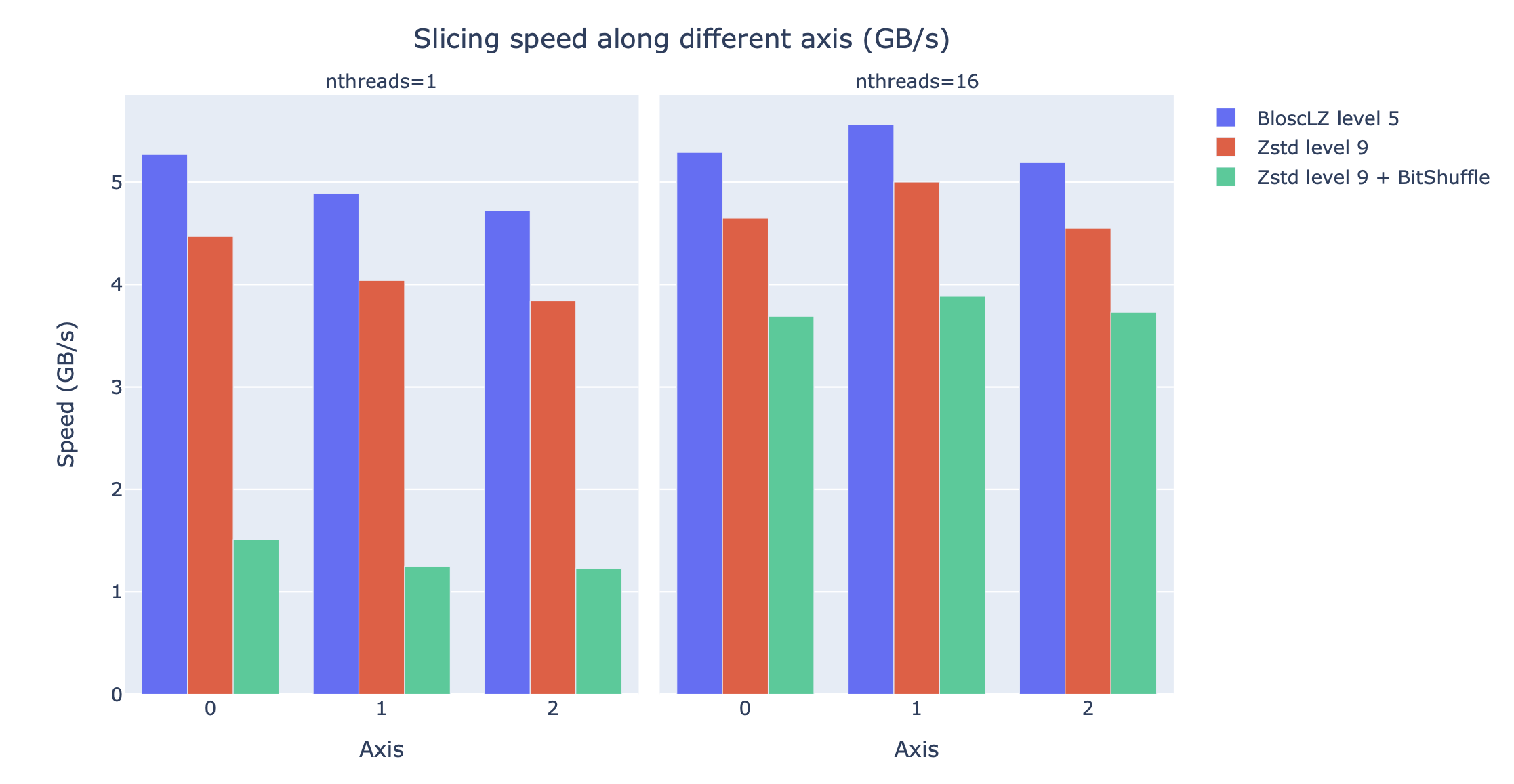
Figure 8:Speed of obtaining multiple multidimensional slices of the Gaia dataset along different axes, for different codecs, filters and different number of threads. The speed is measured in GB/s, so a higher value is better.
These results indicate that the fastest compression is achieved with BloscLZ (compression level 5, no filters), closely followed by Zstd (compression level 9, no filters), exactly as the neural network model predicted. Also, note how the fastest decompression codecs, BloscLZ and also Zstd, are not affected very much by the number of threads used, which means that they are not CPU-bound, so small computers or laptops with low core counts will be able to reach good speeds.
Now, let’s compare the figures above with other libraries that can handle multidimensional data. Figure 9 shows the slicing speed of the 3D array when applying BloscLZ, the best predicted codec for speed, and we compare that speed against other libraries using the same codec but with the previous Blosc1 generation (Zarr and h5py), and also against Blosc2 via the hdf5plugin Silx maintainers (2023) and h5py. Results show that the data can be explored significantly faster using Blosc2 NDim with the BloscLZ codec. It is also interesting to note that the speed of Blosc2 NDim with BloscLZ is not much affected by the number of threads used, which is a welcome surprise, and probably an indication that the internal zero-suppression mechanism inside Blosc2 works efficiently without the need of multi-threading.
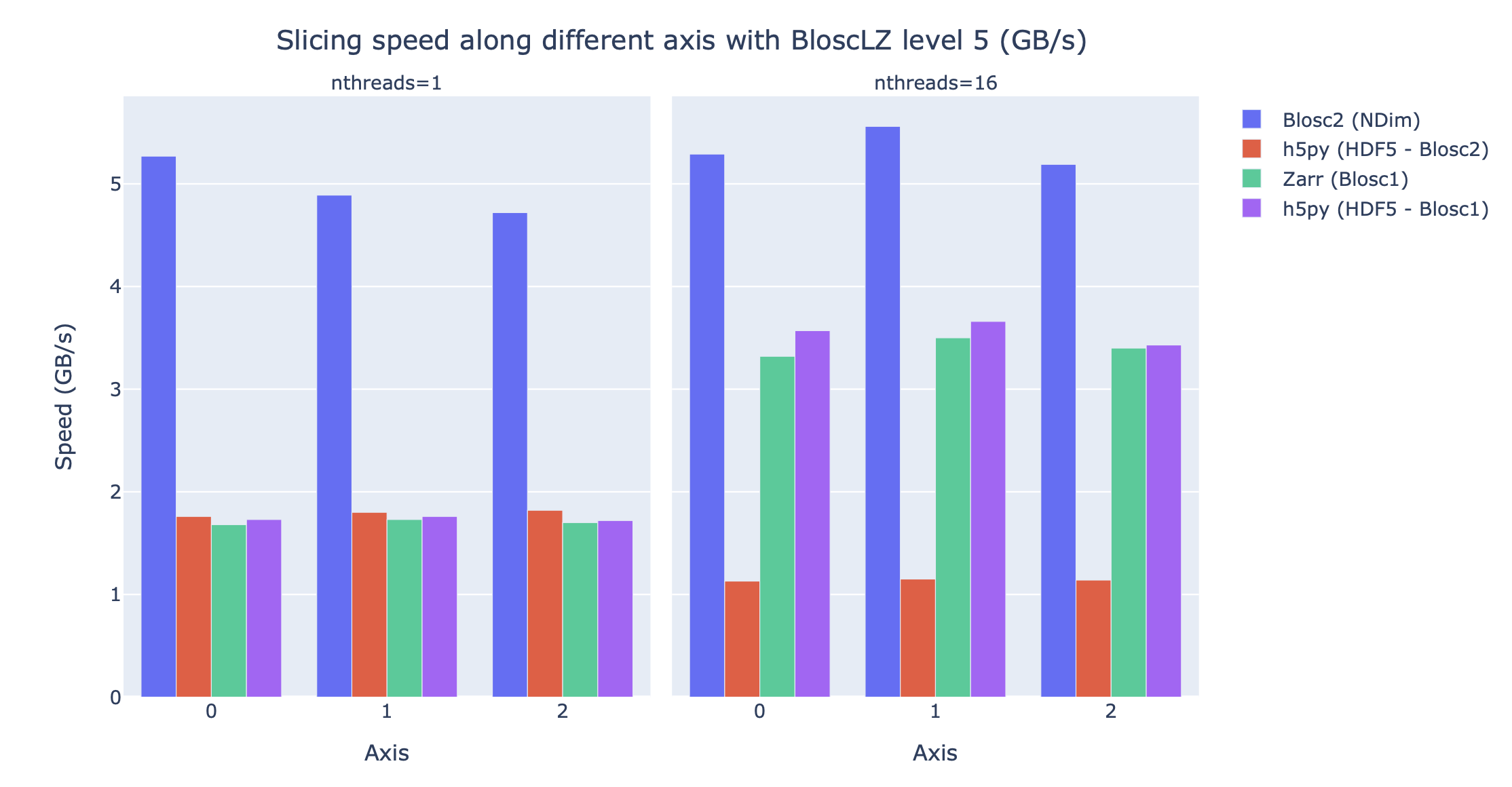
Figure 9:Slicing a section of the Gaia dataset with BloscLZ using different libraries. Note how using one single thread is still quite effective for Blosc2 NDim and BloscLZ.
Regarding compression ratio, Figure 10 shows the results of compressing the Gaia dataset with Blosc2 NDim with BloscLZ and Zstd, and we compare that ratio against other libraries using the same codec but with the previous Blosc1 generation (Zarr and h5py), and also against Blosc2 via the hdf5plugin and h5py. Results show that the data can be compressed significantly better using Blosc2. This is because Blosc2 comes with a new and powerful zero-detection mechanism that is able to efficiently handle and compress the many zeros that are present in the Gaia dataset.
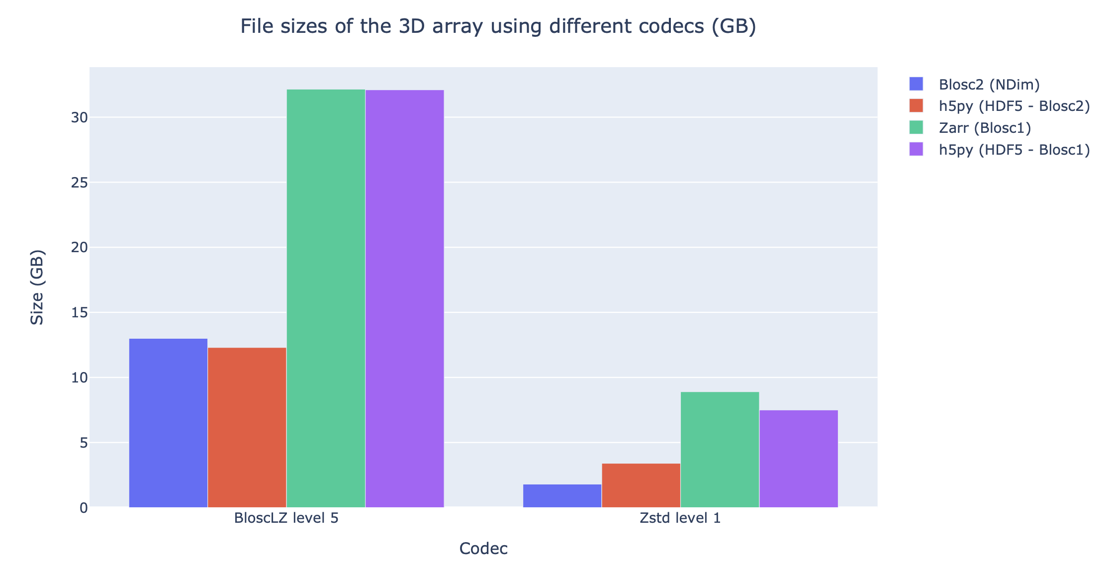
Figure 10:Compressing the Gaia dataset with BloscLZ and Zstd using different libraries. Blosc2 provides significantly better compression ratios than using Blosc1 . Also, note how Zstd compresses much better than BloscLZ.
Ingesting and processing data of Gaia
The raw data of Gaia is stored in CSV files. The coordinates are stored in the gaia_source directory (http://
def load_rawdata(out="gaia.b2nd"):
    dtype = {"ra": np.float32,
             "dec": np.float32,
             "parallax": np.float32}
    barr = None
    for file in glob.glob("gaia-source/*.csv*"):
        # Load raw data
        df = pd.read_csv(
            file,
            usecols=["ra", "dec", "parallax"],
            dtype=dtype, comment='#')
        # Convert to numpy array and remove NaNs
        arr = df.to_numpy()
        arr = arr[~np.isnan(arr[:, 2])]
        if barr is None:
            # Create a new Blosc2 file
            barr = blosc2.asarray(
                arr,
                chunks=(2**20, 3),
                urlpath=out,
                mode="w")
        else:
            # Append to existing Blosc2 file
            barr.resize(
                (barr.shape[0] + arr.shape[0], 3))
            barr[-arr.shape[0]:] = arr
    return barr
Once we have the raw data in a Blosc2 container, we can select the stars in a radius of 10 thousand light years using this function:
def convert_select_data(fin="gaia.b2nd",
                        fout="gaia-ly.b2nd"):
    barr = blosc2.open(fin)
    ra = barr[:, 0]
    dec = barr[:, 1]
    parallax = barr[:, 2]
    # 1 parsec = 3.26 light years
    ly = ne.evaluate("3260 / parallax")
    # Remove ly < 0 and > 10_000
    valid_ly = ne.evaluate(
        "(ly > 0) & (ly < 10_000)")
    ra = ra[valid_ly]
    dec = dec[valid_ly]
    ly = ly[valid_ly]
    # Cartesian x, y, z from spherical ra, dec, ly
    x = ne.evaluate("ly * cos(ra) * cos(dec)")
    y = ne.evaluate("ly * sin(ra) * cos(dec)")
    z = ne.evaluate("ly * sin(dec)")
    # Save to a new Blosc2 file
    out = blosc2.zeros(mode="w", shape=(3, len(x)),
                       dtype=x.dtype, urlpath=fout)
    out[0, :] = x
    out[1, :] = y
    out[2, :] = z
    return out
Finally, we can compute the density of stars in a 3D grid with this script:
R = 1  # resolution of the 3D cells in ly
LY_RADIUS = 10_000  # radius of the sphere in ly
CUBE_SIDE = (2 * LY_RADIUS) // R
MAX_STARS = 1000_000_000  # max number of stars to load

b = blosc2.open("gaia-ly.b2nd")
x = b[0, :MAX_STARS]
y = b[1, :MAX_STARS]
z = b[2, :MAX_STARS]

# Create 3d array.
# Be sure to have enough swap memory (around 8 TB!)
a3d = np.zeros((CUBE_SIDE, CUBE_SIDE, CUBE_SIDE),
               dtype=np.float32)
for i, coords in enumerate(zip(x, y, z)):
    x_, y_, z_ = coords
    a3d[(np.floor(x_) + LY_RADIUS) // R,
        (np.floor(y_) + LY_RADIUS) // R,
        (np.floor(z_) + LY_RADIUS) // R] += 1

# Save 3d array as Blosc2 NDim file
blosc2.asarray(a3d,
               urlpath="gaia-3d.b2nd", mode="w",
               chunks=(250, 250, 250),
               blocks=None,
               )
With that, we have a 3D array of shape 20,000 x 20,000 x 20,000 with the number of stars with a 1 light year resolution. We can visualize the vicinity of our Sun with Plotly Plotly Technologies Inc. (2015) making use of the following code:
import blosc2
import numpy as np
import plotly.express as px

nstars_path = '$HOME/Gaia/gaia-3d-windows-int8.b2nd'
b3d = blosc2.open(nstars_path)
data = b3d[9_975:10_025, 9_975:10_025, 9_975:10_025]
idx = np.indices(data.shape)
fig = px.scatter_3d(x=idx[0, :, :, :].flatten(),
                    y=idx[1, :, :, :].flatten(),
                    z=idx[2, :, :, :].flatten(),
                    size=data[...].flatten())
fig.show()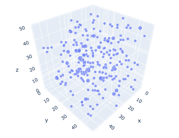
Figure 11:Stars in the vicinity of our Sun (cube of 50 light years). Each point represents a star, and its size represents the number of stars in that location (a cube of 1 x 1 x 1 light year). The maximum amount of stars in a single location for this view is 3 (triple star systems are common).
Figure 11 displays an interactive 3D view of the stars within a 50 x 50 x 50 light-year cube centered around our Sun. This visualization was generated using the code above.
In The Blosc Development Team (2023) you can find the final version of the scripts above, including optimized versions that do not require a machine with more than 32 GB of virtual memory to run.
Conclusions
Working with large, multi-dimensional data cubes can be challenging due to the costly data handling involved. In this document, we demonstrate how the two-partition feature in Blosc2 NDim can help reduce the amount of data movement required when retrieving thin slices of large datasets. Additionally, this feature provides a foundation for leveraging cache hierarchies in modern CPUs.
Blosc2 supports a variety of compression codecs and filters, making it easier to select the most appropriate ones for the dataset being explored. It also supports storage in either memory or on disk, which is crucial for large datasets. Another important feature is the ability to store data in a container format that can be easily shared across different programming languages. Furthermore, Blosc2 has special support for sparse datasets, which greatly improves the compression ratio in this scenario.
We have also shown how the Btune plugin can be used to automatically tune the compression parameters for a given dataset. This is especially useful when we want to compress data efficiently for a tradeoff between compression or decompression speed and compression ratio, but we do not know the best compression parameters beforehand.
In conclusion, we have shown how to utilize the Blosc2 library for storing and processing the Gaia dataset. This dataset serves as a prime example of a large, multi-dimensional dataset that can be efficiently stored and processed using Blosc2 NDim.
Jordi Portell, member of the Gaia Collaboration, has been very helpful in answering many questions about the Gaia dataset, and has also proposed possible explorations of it.
NumFOCUS, a non-profit organization with a mission to promote open practices in research, data, and scientific computing. They have provided steady funds to the Blosc Development Team over the past years.
Huawei, a high-tech company that made a significant and selfless donation to the Blosc project.
Sergio Barrachina, associate professor at University Jaume I, has provided many advice and code during the development of the Btune project.
This work has made use of data from the European Space Agency (ESA) mission Gaia (https://
Copyright © 2023 Blosc et al. This is an open-access article distributed under the terms of the Creative Commons Attribution 3.0 Unported license.
- CPU
- central processing unit
- ESA
- European Space Agency
- SIMD
- single-instruction multiple-data streams
- Francesc Alted. (2010). Why Modern CPUs Are Starving and What Can Be Done About It. Computing in Science and Engineering, 12(2), 68–71.
- Francesc Alted. (2018). Breaking Down Memory Walls.
- The HDF Group. (1997-2023). Hierarchical Data Format, version 5.
- Zarr Developers. (2017-2023). An implementation of chunked, compressed, N-dimensional arrays for Python.
- PyTables developers. (2002-2023). A Python package to manage extremely large amounts of data.
- Francesc Alted and Oscar Guiñón. (2023). Introducing Blosc2 NDim.
- European Space Agency (ESA) and Gaia Data Processing and Analysis Consortium (DPAC). (2023). Gaia Data Release 3. Documentation release 1.2.
- Marta Iborra. (2022). User Defined Pipeline for Python-Blosc2.
- Marta Iborra and Francesc Alted. (2023). Dynamic Plugins in C-Blosc2.
- Silx maintainers. (2023). Set of compression filters for h5py.
- Plotly Technologies Inc. (2015). Collaborative data science. Plotly Technologies Inc.
- The Blosc Development Team. (2023). Scripts for “A Fast Explorer Of The Milky Way” talk.
