EEG-to-fMRI Neuroimaging Cross Modal Synthesis in Python
Abstract
Electroencepholography (EEG) and functional magnetic resonance imaging (fMRI) are two ways of recording brain activity; the former provides good time resolution but poor spatial resolution, while the converse is true for the latter. Recently, deep neural network models have been developed that can synthesize fMRI activity from EEG signals, and vice versa. Because these generative models simulate data, they make it easier for neuroscientists to test ideas about how EEG and fMRI signals relate to each other, and what both signals tell us about how the brain controls behavior. To make it easier for researchers to access these models, and to standardize how they are used, we developed a Python package, EEG-to-fMRI, which provides cross modal neuroimaging synthesis functionalities. This is the first open source software enabling neuroimaging synthesis. Our main focus is for this package to help neuroscience, machine learning, and health care communities. This study gives an in-depth description of this package, along with the theoretical foundations and respective results.
Introduction
Neuronal activity, usually measured through electroencephalography (EEG), is related to haemodynamical activity, measured through functional magnetic resonance imaging (fMRI). The first captures the dynamics of the electrical field, whose source is located from the firing neurons’ action potentials. In its turn, the second measures the blood supply dynamics. These two while being studied simultaneously Shibasaki, 2008Yu et al., 2016He et al., 2018Rojas et al., 2018Bréchet et al., 2019Daly et al., 2019Cury et al., 2020Abreu et al., 2021 differ in many aspects such as: temporal and spatial resolution, brain functions captured, recording and hardware cost. Recently we have seen several studies that use deep neural network models Goodfellow et al., 2016 to learn a mapping from EEG data to and from fMRI data Liu & others, 2019Calhas & Henriques, 2022. These are a type of generative models Murphy, 2012, that sample/synthesize instances from a different data source (instead of a distribution). Such a model could allow health care cost reductions and discoveries of new neuroscience insights on the relationship between these two modalities. Indeed, pathologies that require MRI scans diagnostics benefit from a lower cost EEG assessment, since availability of MRI hardware is very scarce Ogbole et al., 2018. As Python Van Rossum & Drake Jr, 1995 becomes a hub for scientific development Harris et al., 2020Virtanen et al., 2020Abadi et al., 2016 we find the need to provide open source software that provides solutions for EEG to fMRI synthesis, urgent, in order for third party scientific contributions coming from other laboratories to coexist and health care software integration to develop for diagnostic settings. To that end, we provide a description of the open source software EEG-to-fMRI, which originated from an academic scientific project funded by Fundação para a Ciência e Tecnologia, and make publicly available a github repository.
Methods
The mapping function provided in this software is the one proposed by Calhas & Henriques, 2022. It consists on transforming the EEG from a channel by time representation to a channel by time-frequency one, achieved using the short time Fourier transform Allen, 1977 by means of the fast Fourier transform (scipy.fft.fft) available in the SciPy package. The latter corresponds to the second step of the diagram illustrated in Figure 1. In the second step, this representation is then forward through a deep neural network (implemented as a tf.keras.Model), with contributions ranging from Resnet blocks He et al., 2016, an automated machine learning framework Calhas et al., 2022 and Fourier features Tancik et al., 2020. Ultimately, this enables the prediction of an fMRI volume associated with a 26 second segment of an EEG recording.

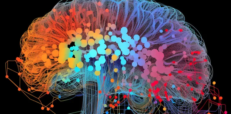
Figure 1:The pipeline of the EEG to fMRI synthesis project consists of processing EEG recordings, that are sourced from a human subject that goes through an EEG recording session, then processing the channel by time signal and taking the short time Fourier transform. The latter, gives us the time frequency representation of the EEG signal. The novelty of this software is that it provides a model that given as input the EEG signal it predicts the corresponding fMRI volume associated with that segment. A video demonstration of the whole pipeline is available on YouTube.
Description
The dependencies of each component are described in an UML diagram. Overall to install the package, the user is required to install the following dependencies: tensorflow 2.9.0, matplotlib 3.5.3, mne 0.23.4, nilearn 0.7.0, tensorflow_probability 0.12.2, tensorflow_determinism 0.3.0, and tensorflow_addons 0.19.0. As seen there is a high dependency in tensorflow related packages. This is due to the whole system provided being built in tensorflow, a library that enables automatic differentiation and is widely used for deep learning model development.
Package modules
This package, as it is provided, has eight main modules:
models: here you will find the code that implements the models for synthesis and classification. The synthesis models are located in the synthesizers.py, where the class EEG_to_fMRI is implemented. This class defines a
tf.keras.Model, composed of two encoders, one for the EEG and another for the fMRI. Additionally, there is a decoder that maps the latent EEG representation, that is the output of the EEG encoder, to the estimate of the fMRI volume associated. The fMRI encoder is defined in the fmri_ae.py file. The task would not be complete without the extrapolation of the synthesis model to a classification task. To that end, two linear classifiers are provided, the ViewLatentContrastiveClassifier and the ViewLatentLikelihoodClassifier, corresponding to a contrastive latent loss and a cross entropy error driven classification, respectively. The extrapolation is made by taking the output of the neural flow that comes from the EEG, that is the EEG encoder and the decoder.layers: this module contains the layers which compose the synthesizer models. It provides five main types of layers. First, the TopographicalAttention computes a self attention mechanism in the channels dimension of the EEG Calhas & Henriques, 2022 that allows the representation to be correctly processed by the convolutional blocks. Second, the ResnetBlock He et al., 2016 implements a residual block composed of convolutional layers. This block allows efficient gradient propagation, by tackling the vanishing gradient phenomena. Third, the FourierFeatures layer projects cosines functions of different shifts and biases to build a latent spectral basis for the prediction of the fMRI volume. Fourth, the DenseVariational is an implementation of the
tf.keras.layers.Denselayer for two-dimensional inputs, whose weights are drawn from gaussian distributions. Last, but not least, we provide the DCT based layers, which implement the discrete cosine transform Ahmed & Natarajan, 1974. These layers are useful for alternative ways of decoding the latent representation of the EEG to produce the desired fMRI volume.regularizers: here the implementation of different regularizers for the synthesizer model is provided. Most importantly in the activity_regularizers.py file is found the OrganizeChannels implementation which can be added in the TopographicalAttention layer, so that the layer does not surpress any channel;
learning: here are implemented the routines for the optimization of the models, namely the losses and the train procedures. The train.py is a generalizable training routine that fits any type of
tf.keras.Modelinstance. Following, the losses.py contain a set of losses that are implemented to train the models provided in the models module. Most importantly, here you will find the mae_cosine for the deterministic versions of the EEG_to_fMRI model, the LaplacianLoss for variational versions, and the ContrastiveClassificationLoss which serves as the cost function for the ViewLatentContrastiveClassifier;explainability: this module contains explainability methods that were employed for the models developed. The implementation for the layer wise relevance propagation Bach et al., 2015 can be found in lrp.py. In particular, since this type of algorithm is not model agnostic, we have the implementation for all the permutations’ of operations that the EEG_to_fMRI model can have;
data: this is maybe the most important module for researchers wanting to try out their collected data with this software. Here all of the functions, that read data and manipulate it as such to allow the efficient training, are implemented. Starting with the eeg_utils.py, where the get_eeg_instance_<DS> function is implemented for a limited set of datasets that participated in the experiments of the associated studies. The <DS> stands for the identifier of the dataset. Currently there are a set of functions implemented for publicly available datasets. Please check the description of the code in the github repository for more details. In the fmri_utils.py file one finds functions of the form get_individuals_paths_<DS>, that have the exact same function as the functions to read EEG recordings, but in this case they read nifti file format. These type of files are the standard format for fMRI recordings. Finally, the data_utils.py and preprocessed_data.py are responsible for concatenating the EEG and fMRI instance pairs, with all the alignments and event synchronization events taken into account, as well as the processing to build
tf.data.Datasetclasses.metrics: in this module are implemented the metrics usually used to evaluate synthesis of generated images, such as the root mean squared error, mean absolute error, structural similarity index measure Wang et al., 2004, among others;
utils: Last but not least, is the utilities module, which provides the user with print functions, configuration of the tensorflow environments and several visualizations that were used in the original studies that developed the package.

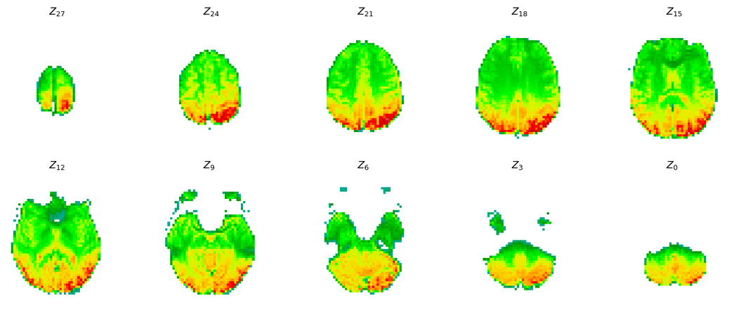
Figure 2:The synthesized signal of fMRI. This is the output visualization when running the code for the classification notebook.
New data integration
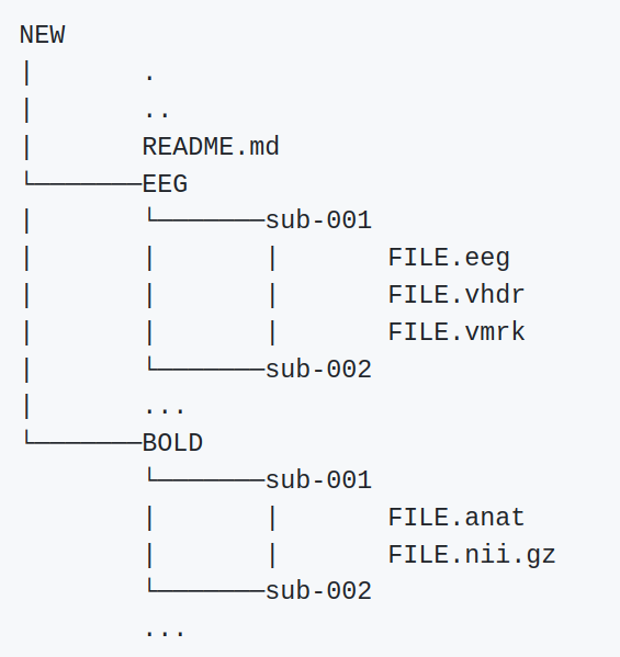
In order to use the software provided for new data, we recommend that the dataset is structured as shown in Figure 3.

Figure 3:Recommended structure of the dataset directory.
If the data is provided as illustrated then the user only has to name the directory of the data as 01. This should suffice for the correct loading of the data. Any type of issue that is encountered for this package should be published as an issue in the official github repository.
Building an EEG to fMRI model
For the user to build an EEG to fMRI model, they have to first import the correct library module and tensorflow.
from tensorflow as tf
from eeg_to_fmri.models.synthesizers
        import EEG_to_fMRI
from eeg_to_fmri.models.synthesizers
        import parameters
from eeg_to_fmri.models.synthesizers
        import na_specification_eeg
from eeg_to_fmri.models.fmri_ae
        import na_specification_fmri
Let us define the size of the EEG representation , the fMRI representation , and the latent representation, for both the EEG and fMRI, that is .
fmri_dim=(64,134,10,1)
fmri_dim=(64,64,30,1)
latent_dim=(7,7,7)
Then, we have to define the parameters for the model, these are provided as a variable in the synthesizers.py.
learning_rate,weight_decay,kernel_size,
stride_size,batch_size,latent_dimension,
n_channels,max_pool,batch_norm,
skip_connections,dropout,
n_stacks,outfilter,local=parameters
Some of these parameters will also be used to define the fMRI encoder. Since the fMRI encoder is a different class, we need to define the initialization parameters.
fmri_parameters=(parameters, latent_dim,
    fmri_dim, kernel_size, stride_size,
    n_channels, max_pool, batch_norm,
    weight_decay, skip_connections,
    n_stacks, True, False,
    outfilter, dropout, None,
    False, na_specification_fmri)
Next, we have all of the parameters necessary to build a simple deterministic version of the EEG to fMRI model.
with tf.device('/CPU:0'):
    model = EEG_to_fMRI(latent_dim, eeg_dim,
        na_specification_eeg, n_channels,
        weight_decay=weight_decay,
        skip_connections=True, batch_norm=True,
        fourier_features=True,
        random_fourier=True,
        topographical_attention=True,
        conditional_attention_style=True,
        conditional_attention_style_prior=False,
        local=True, seed=None,
        fmri_args = fmri_parameters)
The model is built once it is specified the input dimension, this is done through the tf.keras.Layer#build. This will initialize all of the weights of the network.
model.build((None,)+eeg_dim, (None,)+fmri_dim)Cost function and optimization
Regarding the cost function, which is provided in the learning module at the losses.py file, we can specify different metrics that are provided. Take, for instance, the example of using an approximation of the mean absolute error at the output for the fMRI volume prediction , and approximation of the latent representations of the fMRI as proposed by Calhas & Henriques, 2022. This is reduced to the mathematical formula
In terms of code, this is already implemented and can be loaded directly.
from eeg_to_fmri.learning import losses
loss_fn=losses.mae_cosine
The optimizer is already provided in the tensorflow library and its corresponding learning rate is given in the parameters variable.
optimizer=
        tf.keras.optimizers.Adam(learning_rate)
Training the model requires an input, the EEG , and an output, the fMRI . The architecture processes both the EEG and fMRI, producing the latent representation for both. Proceeding the latent EEG representation, , is fed to the decoder which estimates the fMRI .
def apply_gradient(model, optimizer, loss_fn,
    x, y, return_logits=False, call_fn=None):
    with tf.GradientTape(persistent=True) as
                                        tape:
        logits=model(x, y, training=True)
        regularization=0.
        if(len(model.losses)):
            regularization=
                tf.math.add_n(model.losses)
        loss=loss_fn(y, logits)+regularization
    gradients=tape.gradient(loss,
            model.trainable_variables)
    optimizer.apply_gradients(zip(gradients,
        model.trainable_variables))
    return tf.reduce_mean(loss)
The training routine functions are found in the learning module. The function apply_gradient computes the forward and backward pass of the neural network. Note that the input of the EEG_to_fMRI model is composed of two tensors, the EEG and fMRI, which is the reason why one gives the model both x and y. The loss computes both the estimation of the fMRI according to the mean absolute error (MAE) and the cosine distance between the latent representations. Regularization terms, such as weight decay and other activity regularizers that may or may not participate in the model, are also added to the loss. The loss function used for the synthesis task, the one used in Calhas & Henriques, 2022, is the MAE and the cosine distance. This loss function is defined in the learning module, found at the losses.py file. This loss receives a tf.Tensor object, y_true, and a list of tf.Tensor. The list of tensors contains the outputs of the neural network that should be approximate the ground truth. The first element of the list is the estimated fMRI volume and the second and third items are the latent EEG and fMRI representations, respectively.
def mae_cosine(y_true, y_pred):
    return tf.reduce_mean(
        tf.math.abs(y_pred[0] - y_true),
        axis=(1,2,3)) +
        cosine(y_pred[1], y_pred[2])
At test time, the EEG_to_fMRI model can discard the fMRI input. To that end, only the decoder attribute is called, which is composed of the EEG encoder and the decoder.
def call(self, x1, x2):
    if(self.training):
        return [self.decoder(x1),
            self.eeg_encoder(x1),
            self.fmri_encoder(x2)]

    return self.decoder(x1)
Note that, the pretrained_EEG_to_fMRI class processes a pretrained model of the type EEG_to_fMRI and builds a new model that only processes EEG and outputs an fMRI prediction given the representation learned. This class is built to be then appended with a classifier, that can be either a ViewLatentContrastiveClassifier or a ViewLatentLikelihoodClassifier.
Examples
In this section, we walk through the examples given in jupyter notebooks.
Synthesis
We provide a compressed version of the dataset of Deligianni et al., 2014. Users can directly execute the code and have both the python package, as well as the dataset, setup in a google colab environment. The flow of execution has been already described. In the end a synthesized fMRI is shown, as illustrated in Figure 2. This image is built using the viz_utils.py. The user can find metrics for synthesis evaluation in eeg_to_fmri.metrics.quantitative_metrics. We report results from the Calhas & Henriques, 2022 study on the NODDI dataset Deligianni et al., 2014. An example with a reduced dataset is available in this synthesis notebook. The best model, which used the configuration of the eeg_to_fmri.models.synthesizers.EEG_to_fMRI achieved 0.3972 RMSE and 0.4613 SSIM. This constitutes the state-of-the-art for this task and provides a view that can be applied in EEG only datasets for classification task.
Classification

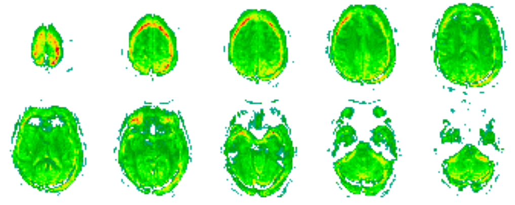
Figure 4:Output of the predicted fMRI when given an EEG representation. Note that, due to the EEG encoder being optimized towards classifying the data according to the groups of individuals defined, e.g. schizophrenic and healthy controls, the decoder (that has the parameters frozen) gives a slightly altered representation. This change is seen in the produced fMRI, where activity beyond the limit of the human scalp is reported. Please recall Figures 1 and 2 to directly compare with an fMRI representation without these flaws.
We also provide a compressed version of the dataset of Padée & others, 2022. This example, available in this classification notebook, is based on a publicly available dataset that contains individuals diagnosed with schizophrenia and healthy controls. The whole goal of the project is to be applied in an health care setting and to this end we employ an end to end software solution. The whole software package is able to synthesize fMRI and adapt to a classification setting, that given EEG recordings outputs a set of probabilities for each group of people considered in the dataset.
Collaboration
Ultimately, the goal of this package is to collect, in one package, methods for EEG to fMRI synthesis. We welcome contributions from authors of related work such as Liu & others, 2019. In the future, we plan to add a module or example folder with implementations of these approaches, so that other research groups can easily access them and reproduce key results.
On a higher level, this software is encouraged for testing its applicability in health care settings. The impact, that such mappings from EEG to fMRI, would have on society is enormous, given that the diagnostic is faithful. Take for instance the example of the MRI machine density across the African continent. In the worst case scenario, Nigeria has a density of 0.33 MRI machines per million people, according to Ogbole et al., 2018. To let that sink in, imagine having to wait in a line of 3 million people to get a diagnostic exam. This type of waiting bottleneck impacts greatly the development of diseases for the worse. Countries in such conditions would greatly benefit from contributions that further advance this scientific field. Even fortunate countries, whose economy thrives, that are able to provide their populations with a good ratio of MRI machines, they still have small portions of the population who live in remote areas. These people find it hard to get quality health care, without having to travel significant distances.
Conclusion
This is the first package, to the best of our knowledge, that provides a machine learning oriented synthesis between functional neuroimaging modalities (EEG and fMRI). It is targeted to help the neuroscience community, in tasks such as modality augmentation, resolution enhancement, neuroimaging explainability techniques, among others. We hope to motivate researchers, scientists, and software developers to contribute to this package which we have been so passionate about throughout the last years.
This work was supported by national funds through Fundação para a Ciência e Tecnologia under the PhD Grant SFRH/BD/5762/2020 to David Calhas.
Copyright © 2023 Calhas. This is an open-access article distributed under the terms of the Creative Commons Attribution 3.0 Unported license.
- EEG
- electroencephalography
- fMRI
- functional magnetic resonance imaging
- MAE
- mean absolute error
- MRI
- magnetic resonance imaging
- RMSE
- root mean squared error
- Shibasaki, H. (2008). Human brain mapping: hemodynamic response and electrophysiology. Clinical Neurophysiology, 119(4), 731–743. 10.1016/j.clinph.2007.10.026
- Yu, Q., Wu, L., Bridwell, D. A., Erhardt, E. B., Du, Y., He, H., Chen, J., Liu, P., Sui, J., Pearlson, G., & others. (2016). Building an EEG-fMRI multi-modal brain graph: a concurrent EEG-fMRI study. Frontiers in Human Neuroscience, 10, 476. 10.3389/fnhum.2016.00476
- He, Y., Steines, M., Sommer, J., Gebhardt, H., Nagels, A., Sammer, G., Kircher, T. T. J., & Straube, B. (2018). Spatial–temporal dynamics of gesture–speech integration: a simultaneous EEG-fMRI study. Brain Structure and Function, 223, 3073–3089. 10.1007/s00429-018-1674-5
- Rojas, G. M., Alvarez, C., Montoya, C. E., de la Iglesia-Vayá, M., Cisternas, J. E., & Gálvez, M. (2018). Study of resting-state functional connectivity networks using EEG electrodes position as seed. Frontiers in Neuroscience, 12, 235. 10.3389/fnins.2018.00235
- Bréchet, L., Brunet, D., Birot, G., Gruetter, R., Michel, C. M., & Jorge, J. (2019). Capturing the spatiotemporal dynamics of self-generated, task-initiated thoughts with EEG and fMRI. Neuroimage, 194, 82–92. 10.1016/j.neuroimage.2019.03.029
- Daly, I., Williams, D., Hwang, F., Kirke, A., Miranda, E. R., & Nasuto, S. J. (2019). Electroencephalography reflects the activity of sub-cortical brain regions during approach-withdrawal behaviour while listening to music. Scientific Reports, 9(1), 1–22. 10.1038/s41598-019-45105-2
- Cury, C., Maurel, P., Gribonval, R., & Barillot, C. (2020). A sparse EEG-informed fMRI model for hybrid EEG-fMRI neurofeedback prediction. Frontiers in Neuroscience, 13, 1451. 10.3389/fnins.2019.01451
- Abreu, R., Jorge, J., Leal, A., Koenig, T., & Figueiredo, P. (2021). EEG microstates predict concurrent fMRI dynamic functional connectivity states. Brain Topography, 34(1), 41–55. 10.1007/s10548-020-00805-1
- Goodfellow, I., Bengio, Y., & Courville, A. (2016). Deep learning. MIT press.
- Liu, X., & others. (2019). A convolutional neural network for transcoding simultaneously acquired EEG-fMRI data. NER. 10.1109/ner.2019.8716994
- Calhas, D., & Henriques, R. (2022). EEG to fMRI Synthesis Benefits from Attentional Graphs of Electrode Relationships. arXiv Preprint arXiv:2203.03481. 10.48550/arXiv.2203.03481
- Murphy, K. P. (2012). Machine learning: a probabilistic perspective. MIT press.
- Ogbole, G. I., Adeyomoye, A. O., Badu-Peprah, A., Mensah, Y., & Nzeh, D. A. (2018). Survey of magnetic resonance imaging availability in West Africa. Pan African Medical Journal, 30(1). 10.11604/pamj.2018.30.240.14000
- Van Rossum, G., & Drake Jr, F. L. (1995). Python tutorial. Centrum voor Wiskunde en Informatica Amsterdam, The Netherlands.
- Harris, C. R., Millman, K. J., Van Der Walt, S. J., Gommers, R., Virtanen, P., Cournapeau, D., Wieser, E., Taylor, J., Berg, S., Smith, N. J., & others. (2020). Array programming with NumPy. Nature, 585(7825), 357–362. 10.1038/s41586-020-2649-2
