
Pylira: deconvolution of images in the presence of Poisson noise
Abstract
All physical and astronomical imaging observations are degraded by the finite angular resolution of the camera and telescope systems. The recovery of the true image is limited by both how well the instrument characteristics are known and by the magnitude of measurement noise. In the case of a high signal to noise ratio data, the image can be sharpened or “deconvolved” robustly by using established standard methods such as the Richardson-Lucy method. However, the situation changes for sparse data and the low signal to noise regime, such as those frequently encountered in X-ray and gamma-ray astronomy, where deconvolution leads inevitably to an amplification of noise and poorly reconstructed images. However, the results in this regime can be improved by making use of physically meaningful prior assumptions and statistically principled modeling techniques. One proposed method is the LIRA algorithm, which requires smoothness of the reconstructed image at multiple scales. In this contribution, we introduce a new python package called Pylira, which exposes the original C implementation of the LIRA algorithm to Python users. We briefly describe the package structure, development setup and show a Chandra as well as Fermi-LAT analysis example.
Introduction
Any physical and astronomical imaging process is affected by the limited angular resolution of the instrument or telescope. In addition, the quality of the resulting image is also degraded by background or instrumental measurement noise and non-uniform exposure. For short wavelengths and associated low intensities of the signal, the imaging process consists of recording individual photons (often called “events”) originating from a source of interest. This imaging process is typical for X-ray and gamma-ray telescopes, but images taken by magnetic resonance imaging or fluorescence microscopy show Poisson noise too. For each individual photon, the incident direction, energy and arrival time is measured. Based on this information, the event can be binned into two dimensional data structures to form an actual image.
As a consequence of the low intensities associated to the recording of individual events, the measured signal follows Poisson statistics. This imposes a non-linear relationship between the measured signal and true underlying intensity as well as a coupling of the signal intensity to the signal variance. Any statistically correct post-processing or reconstruction method thus requires a careful treatment of the Poisson nature of the measured image.
To maximise the scientific use of the data, it is often desired to correct the degradation introduced by the imaging process. Besides correction for non-uniform exposure and background noise this also includes the correction for the “blurring” introduced by the point spread function (PSF) of the instrument. Where the latter process is often called “deconvolution”. Depending on whether the PSF of the instrument is known or not, one distinguishes between the “blind deconvolution” and “non blind deconvolution” process. For astronomical observations, the PSF can often either be simulated, given a model of the telescope and detector, or inferred directly from the data by observing far distant objects, which appear as a point source to the instrument.
While in other branches of astronomy deconvolution methods are already part of the standard analysis, such as the CLEAN algorithm for radio data, developed by Hogbom (1974), this is not the case for X-ray and gamma-ray astronomy. As any deconvolution method aims to enhance small-scale structures in an image, it becomes increasingly hard to solve for the regime of low signal-to-noise ratio, where small-scale structures are more affected by noise.
The Deconvolution Problem
Basic Statistical Model
Assuming the data in each pixel in the recorded counts image follows a Poisson distribution, the total likelihood of obtaining the measured image from a model image of the expected counts with pixels is given by:
By taking the logarithm, dropping the constant terms and inverting the sign one can transform the product into a sum over pixels, which is also often called the Cash Cash, 1979 fit statistics:
Where the expected counts are given by the convolution of the true underlying flux distribution with the PSF :
This operation is often called “forward modelling” or “forward folding” with the instrument response.
Richardson Lucy (RL)
To obtain the most likely value of given the data, one searches a maximum of the total likelihood function, or equivalently a of minimum . This high dimensional optimization problem can e.g., be solved by a classic gradient descent approach. Assuming the pixels values of the true image as independent parameters, one can take the derivative of Eq. 2 with respect to the individual . This way one obtains a rule for how to update the current set of pixels in each iteration of the optimization:
Where α is a factor to define the step size. This method is in general
equivalent to the gradient descent and backpropagation methods used in modern machine
learning techniques. This basic principle of solving the deconvolution problem for
images with Poisson noise was proposed by Richardson (1972) and Lucy (1974).
Their method, named after the original authors, is often known as the Richardson & Lucy (RL)
method. It was shown by Richardson (1972) that this converges to a maximum
likelihood solution of Eq. 2. A Python implementation of the standard RL method
is available e.g. in the Scikit-Image package Walt et al., 2014.
Instead of the iterative, gradient descent based optimization it is also possible to sample from the posterior distribution using a simple Metropolis-Hastings Hastings, 1970 approach and uniform prior. This is demonstrated in one of the Pylira online tutorials (Introduction to Deconvolution using MCMC Methods).
RL Reconstruction Quality
While technically the RL method converges to a maximum likelihood solution, it mostly still results in poorly restored images, especially if extended emission regions are present in the image. The problem is illustrated in Figure 1 using a simulated example image. While for a low number of iterations, the RL method still results in a smooth intensity distribution, the structure of the image decomposes more and more into a set of point-like sources with growing number of iterations.
Because of the PSF convolution, an extended emission region can decompose into multiple nearby point sources and still lead to good model prediction, when compared with the data. Those almost equally good solutions correspond to many narrow local minima or “spikes” in the global likelihood surface. Depending on the start estimate for the reconstructed image the RL method will follow the steepest gradient and converge towards the nearest narrow local minimum. This problem has been described by multiple authors, such as Perry & Reeves (1994) and Fish et al. (1995).
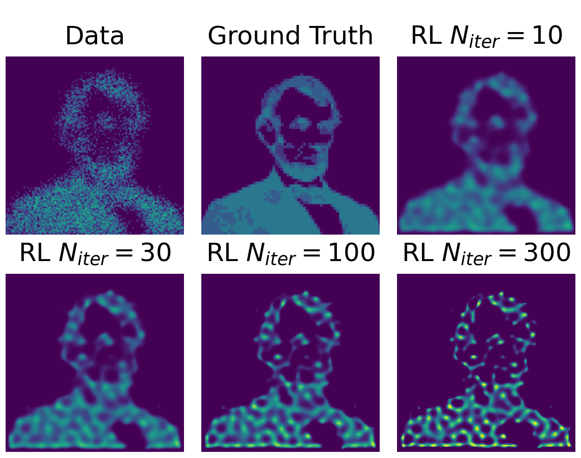
Figure 1:The images show the result of the RL algorithm applied to a simulated example dataset
with varying numbers of iterations. The image in the upper left shows the simulated
counts. Those have been derived from the ground truth (upper mid) by convolving with
a Gaussian PSF of width and applying Poisson noise to
it. The illustration uses the implementation of the RL algorithm from the Scikit-Image
package Walt et al., 2014.
Multi-Scale Prior & LIRA
One solution to this problem was described in Esch et al. (2004) and Connors et al. (2011). First, the simple forward folded model described in Eq. 3 can be extended by taking into account the non-uniform exposure and an additional known background component :
The background can be more generally understood as a “baseline” image and thus include known structures, which are not of interest for the deconvolution process. E.g., a bright point source to model the core of an AGN while studying its jets.
Second, the authors proposed to extend the Poisson log-likelihood function (Equation Eq. 2) by a log-prior term that controls the smoothness of the reconstructed image on multiple spatial scales. Starting from the full resolution, the image pixels are collected into 2 by 2 groups . The four pixel values associated with each group are divided by their sum to obtain a grid of “split proportions” with respect to the image down-sized by a factor of two along both axes. This process is repeated using the down sized image with pixel values equal to the sums over the 2 by 2 groups from the full-resolution image, and the process continues until the resolution of the image is only a single pixel, containing the total sum of the full-resolution image. This multi-scale representation is illustrated in Figure 2.
For each of the 2x2 groups of the re-normalized images a Dirichlet distribution is introduced as a prior:
and multiplied across all 2x2 groups and resolution levels . For each resolution level a smoothing parameter is introduced. These hyper-parameters can be interpreted as having an information content equivalent of adding “hallucinated” counts in each grouping. This effectively results in a smoothing of the image at the given resolution level. The distribution of α values at each resolution level is the further described by a hyper-prior distribution:
Resulting in a fully hierarchical Bayesian model. A more complete and detailed description of the prior definition is given in Esch et al. (2004).
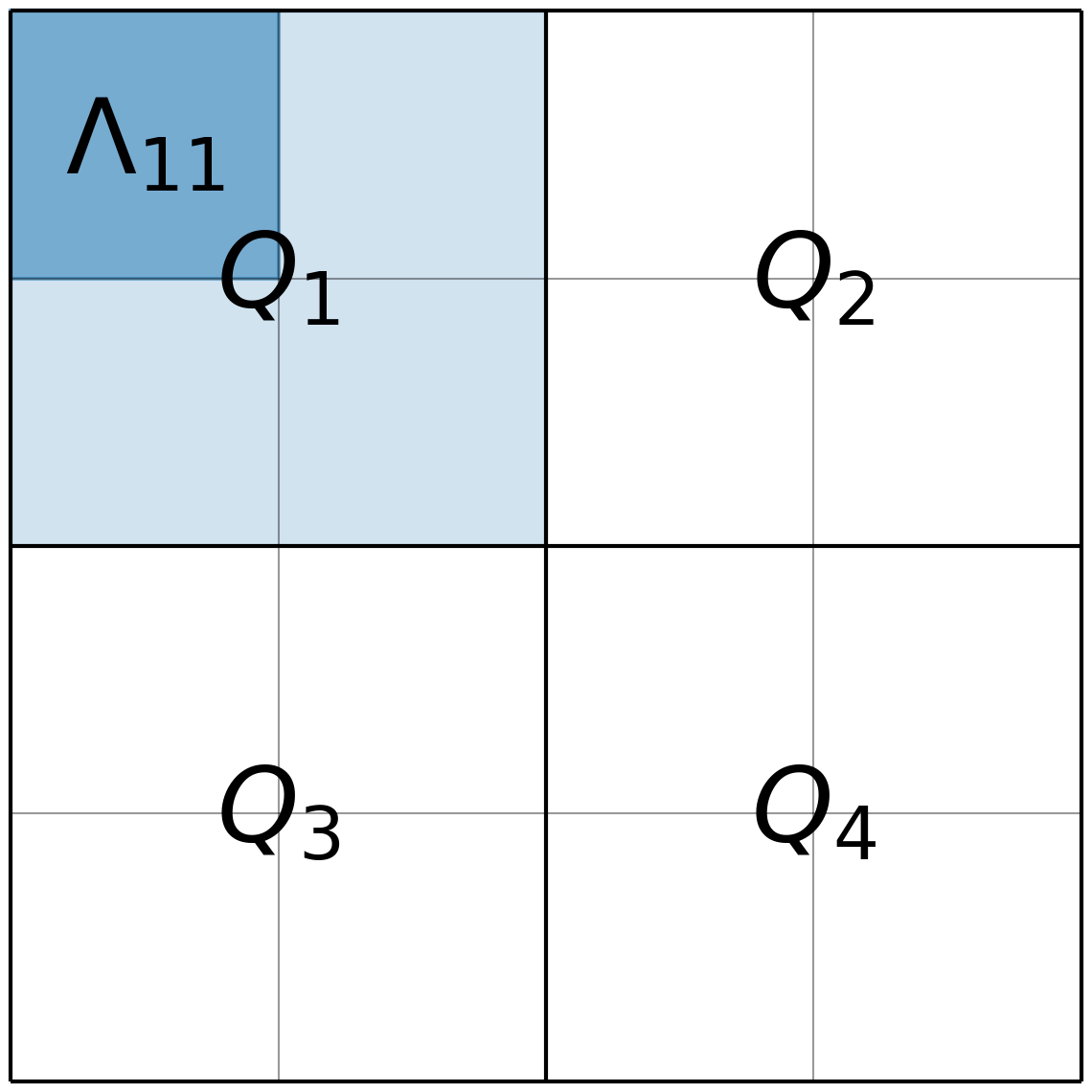
Figure 2:The image illustrates the multi-scale decomposition used in the LIRA prior for a 4x4 pixels example image. Each quadrant of 2x2 sub-images is labelled with . The sub-pixels in each quadrant are labelled .
The problem is then solved by using a Gibbs MCMC sampling approach. After a “burn-in” phase the sampling process typically reaches convergence and starts sampling from the posterior distribution. The reconstructed image is then computed as the mean of the posterior samples. As for each pixel a full distribution of its values is available, the information can also be used to compute the associated error of the reconstructed value. This is another main advantage over RL or Maxium A-Postori (MAP) algorithms.
The Pylira Package
Dependencies & Development
The Pylira package is a thin Python wrapper around the original LIRA implementation provided by
the authors of Connors et al. (2011). The original algorithm was implemented in C and made available
as a package for the R Language R Core Team, 2020. Thus the implementation depends on the RMath library,
which is still a required dependency of Pylira.
The Python wrapper was built using the Pybind11 Jakob et al., 2017 package, which allows to reduce
the code overhead introduced by the wrapper to a minimum. For the data handling, Pylira
relies on Numpy Harris et al., 2020 arrays for the serialisation to the FITS data format
on Astropy Collaboration, 2018. The (interactive)
plotting functionality is achieved via Matplotlib Hunter, 2007 and Ipywidgets community, 2015,
which are both optional dependencies. Pylira is openly developed on Github at https://
Installation
Pylira is available via the Python package index (pypi.org), currently at version 0.1. As Pylira still depends on the RMath library, it is required to install this first. So the recommended way to install Pylira is on MacOS is:
1 2$ brew install r $ pip install pylira
On Linux the RMath dependency can be installed using standard package managers. For example on Ubuntu, one would do
1 2$ sudo apt-get install r-base-dev r-base r-mathlib $ pip install pylira
For more detailed instructions see Pylira installation instructions.
API & Subpackages
Pylira is structured in multiple sub-packages. The pylira.src module contains the original
C implementation and the Pybind11 wrapper code. The pylira.core sub-package
contains the main Python API, pylira.utils includes utility functions for
plotting and serialisation. And pylira.data implements multiple pre-defined
datasets for testing and tutorials.
Analysis Examples
Simple Point Source
Pylira was designed to offer a simple Python class based user interface, which allows for a short learning curve of using the package for users who are familiar with Python in general and more specifically with Numpy. A typical complete usage example of the Pylira package is shown in the following:
1 2 3 4 5 6 7 8 9 10 11 12 13 14 15 16 17 18 19 20 21 22 23 24 25 26 27 28import numpy as np from pylira import LIRADeconvolver from pylira.data import point_source_gauss_psf # create example dataset data = point_source_gauss_psf() # define initial flux image data["flux_init"] = data["flux"] deconvolve = LIRADeconvolver( n_iter_max=3_000, n_burn_in=500, alpha_init=np.ones(5) ) result = deconvolve.run(data=data) # plot pixel traces, result shown in Figure 3 result.plot_pixel_traces_region( center_pix=(16, 16), radius_pix=3 ) # plot pixel traces, result shown in Figure 4 result.plot_parameter_traces() # finally serialise the result result.write("result.fits")
The main interface is exposed via the LIRADeconvolver class, which takes the configuration of
the algorithm on initialisation. Typical configuration parameters include the total number of
iterations n_iter_max and the number of “burn-in” iterations, to be excluded from the
posterior mean computation. The data, represented by a simple Python dict data structure,
contains a "counts", "psf" and optionally "exposure" and "background" array.
The dataset is then passed to the LIRADeconvolver.run() method to execute the deconvolution.
The result is a LIRADeconvolverResult object, which features the possibility to write the
result as a FITS file, as well as to inspect the result with diagnostic plots. The result of
the computation is shown in the left panel of Figure 3.
Diagnostic Plots
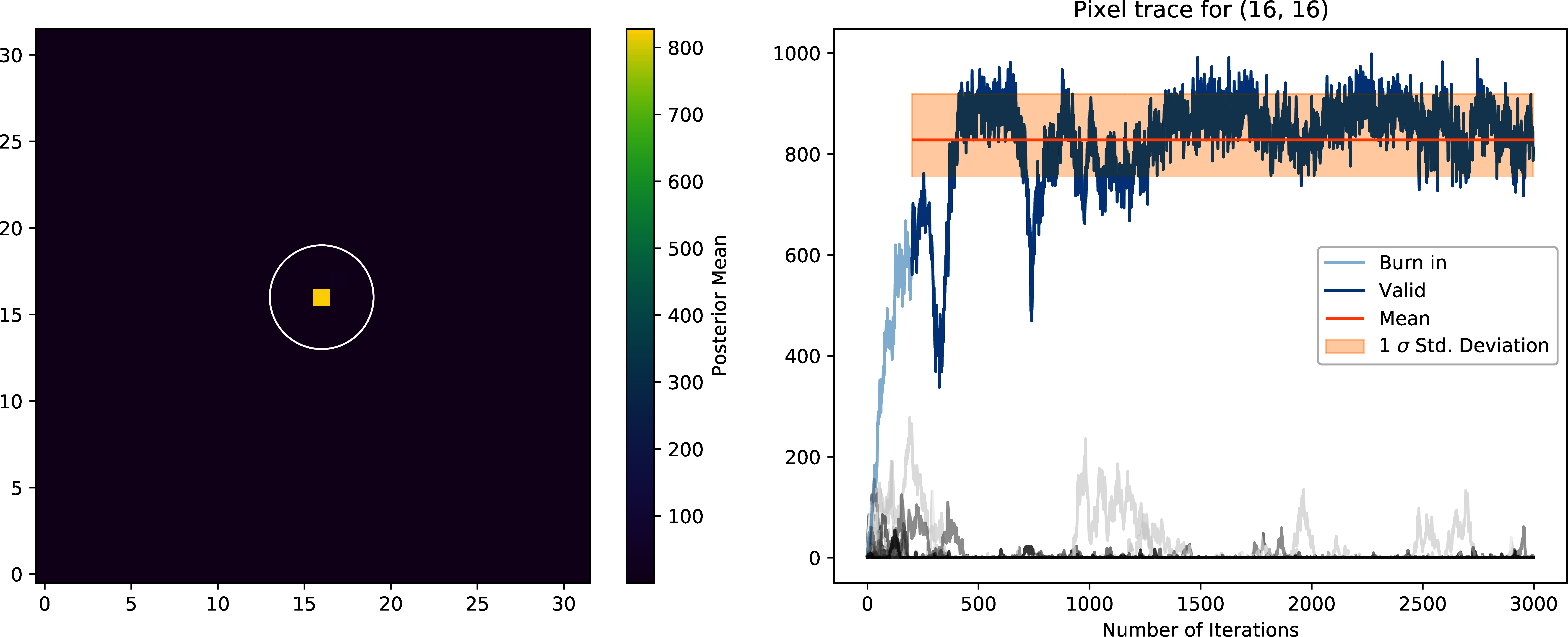
Figure 3:The curves show the traces of value the pixel of interest for a simulated point source and its neighboring pixels (see code example). The image on the left shows the posterior mean. The white circle in the image shows the circular region defining the neighboring pixels. The blue line on the right plot shows the trace of the pixel of interest. The solid horizontal orange line shows the mean value (excluding burn-in) of the pixel across all iterations and the shaded orange area the error region. The burn in phase is shown in transparent blue and ignored while computing the mean. The shaded gray lines show the traces of the neighboring pixels.
To validate the quality of the results Pylira provides many built-in diagnostic plots. One of these diagnostic plot is shown in the right panel of Figure 3. The plot shows the image sampling trace for a single pixel of interest and its surrounding circular region of interest. This visualisation allows the user to assess the stability of a small region in the image e.g. an astronomical point source during the MCMC sampling process. Due to the correlation with neighbouring pixels, the actual value of a pixel might vary in the sampling process, which appears as “dips” in the trace of the pixel of interest and anti-correlated “peaks” in the one or mutiple of the surrounding pixels. In the example a stable state of the pixels of interest is reached after approximately 1000 iterations. This suggests that the number of burn-in iterations, which was defined beforehand, should be increased.
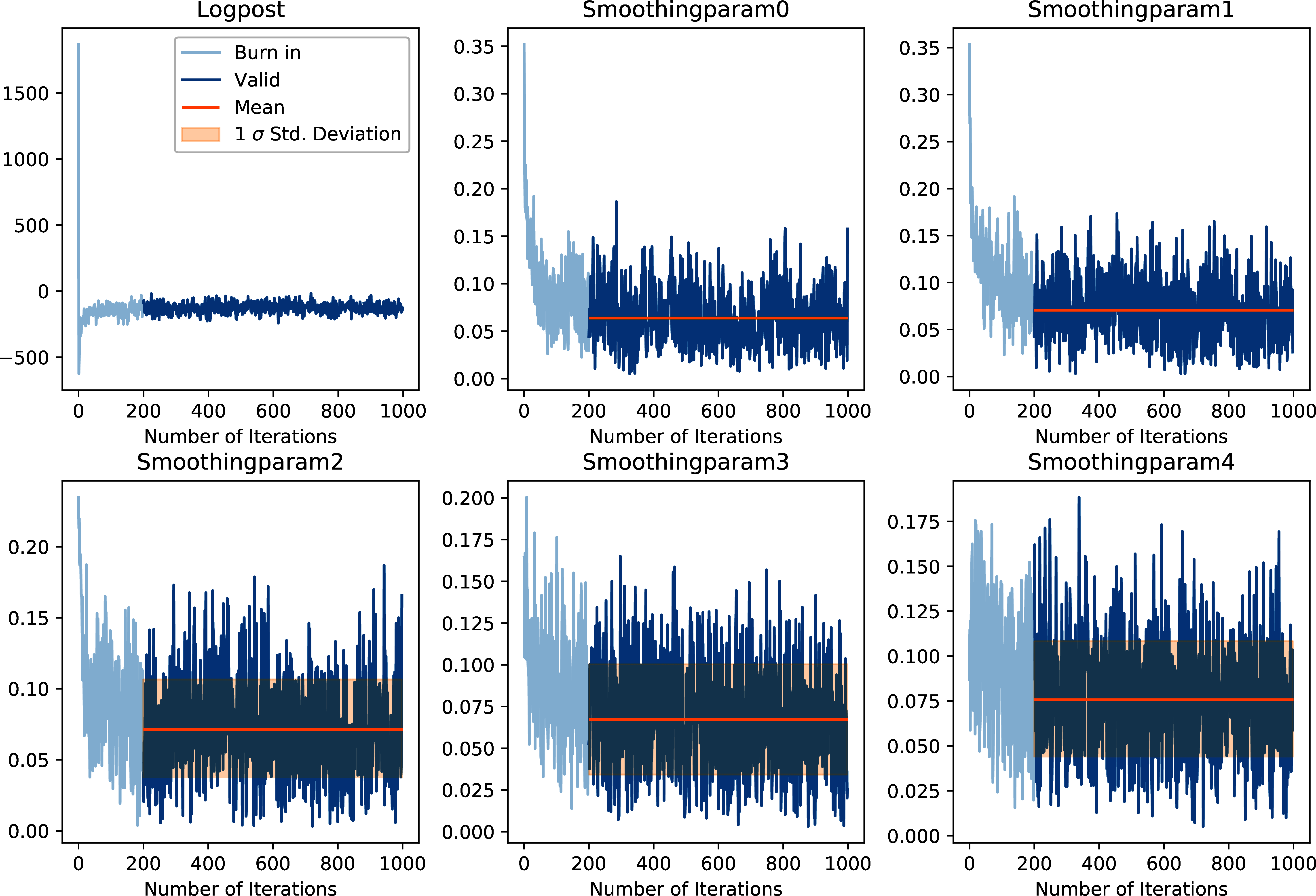
Figure 4:The curves show the traces of the log posterior value as well as traces of the values of the prior parameter values. The SmoothingparamN parameters correspond to the smoothing parameters per multi-scale level. The solid horizontal orange lines show the mean value, the shaded orange area the error region. The burn in phase is shown transparent and ignored while estimating the mean.
Pylira relies on an MCMC sampling approach to sample a series of reconstructed images from the posterior likelihood defined by Eq. 2. Along with the sampling, it marginalises over the smoothing hyper-parameters and optimizes them in the same process. To diagnose the validity of the results it is important to visualise the sampling traces of both the sampled images as well as hyper-parameters.
Figure 4 shows another typical diagnostic plot created by the code example above. In a multi-panel figure, the user can inspect the traces of the total log-posterior as well as the traces of the smoothing parameters. Each panel corresponds to the smoothing hyper parameter introduced for each level of the multi-scale representation of the reconstructed image. The figure also shows the mean value along with the error region. In this case, the algorithm shows stable convergence after a burn-in phase of approximately 200 iterations for the log-posterior as well as all of the multi-scale smoothing parameters.
Astronomical Analysis Examples
Both in the X-ray as well as in the gamma-ray regime, the Galactic Center is a complex emission region. It shows point sources, extended sources, as well as underlying diffuse emission and thus represents a challenge for any astronomical data analysis.
Chandra is a space-based X-ray observatory, which has been in operation since 1999. It consists of nested cylindrical paraboloid and hyperboloid surfaces, which form an imaging optical system for X-rays. In the focal plane, it has multiple instruments for different scientific purposes. This includes a high-resolution camera (HRC) and an Advanced CCD Imaging Spectrometer (ACIS). The typical angular resolution is 0.5 arcsecond and the covered energy ranges from 0.1 - 10 keV.
Figure 5 shows the result of the Pylira algorithm applied to Chandra data of the Galactic Center region between 0.5 and 7 keV. The PSF was obtained from simulations using the simulate_psf tool from the official Chandra science tools ciao 4.14 Fruscione et al., 2006. The algorithm achieves both an improved spatial resolution as well as a reduced noise level and higher contrast of the image in the right panel compared to the unprocessed counts data shown in the left panel.
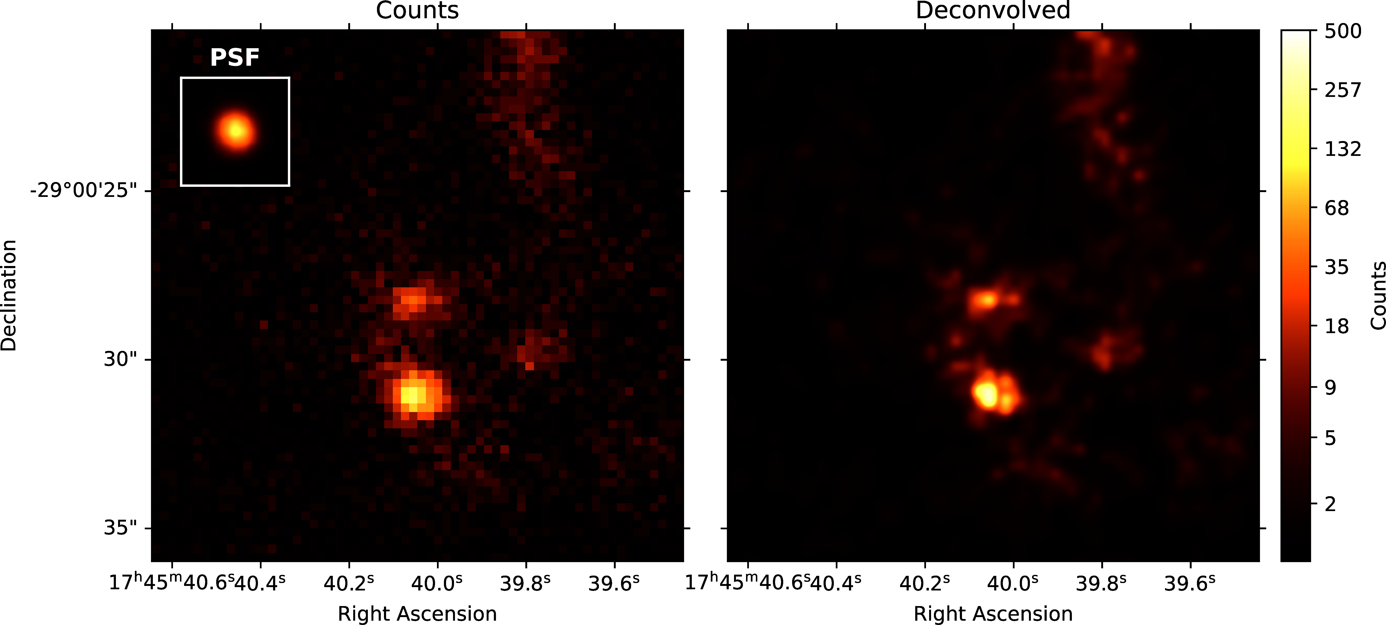
Figure 5:Pylira applied to Chandra ACIS data of the Galactic Center region, using the observation IDs 4684 and 4684. The image on the left shows the raw observed counts between 0.5 and 7 keV. The image on the right shows the deconvolved version. The LIRA hyperprior values were chosen as ms_al_kap1=1, ms_al_kap2=0.02, ms_al_kap3=1. No baseline background model was included.
As a second example, we use data from the Fermi Large Area Telescope (LAT). The Fermi-LAT is a satellite-based imaging gamma-ray detector, which covers an energy range of 20 MeV to >300 GeV. The angular resolution varies strongly with energy and ranges from 0.1 to >10 degree [1].
Figure 6 shows the result of the Pylira algorithm applied to Fermi-LAT data above 1 GeV to the region around the Galactic Center. The PSF was obtained from simulations using the gtpsf tool from the official Fermitools v2.0.19 Fermi Science Support Development Team, 2019. First, one can see that the algorithm achieves again a considerable improvement in the spatial resolution compared to the raw counts. It clearly resolves multiple point sources left to the bright Galactic Center source.
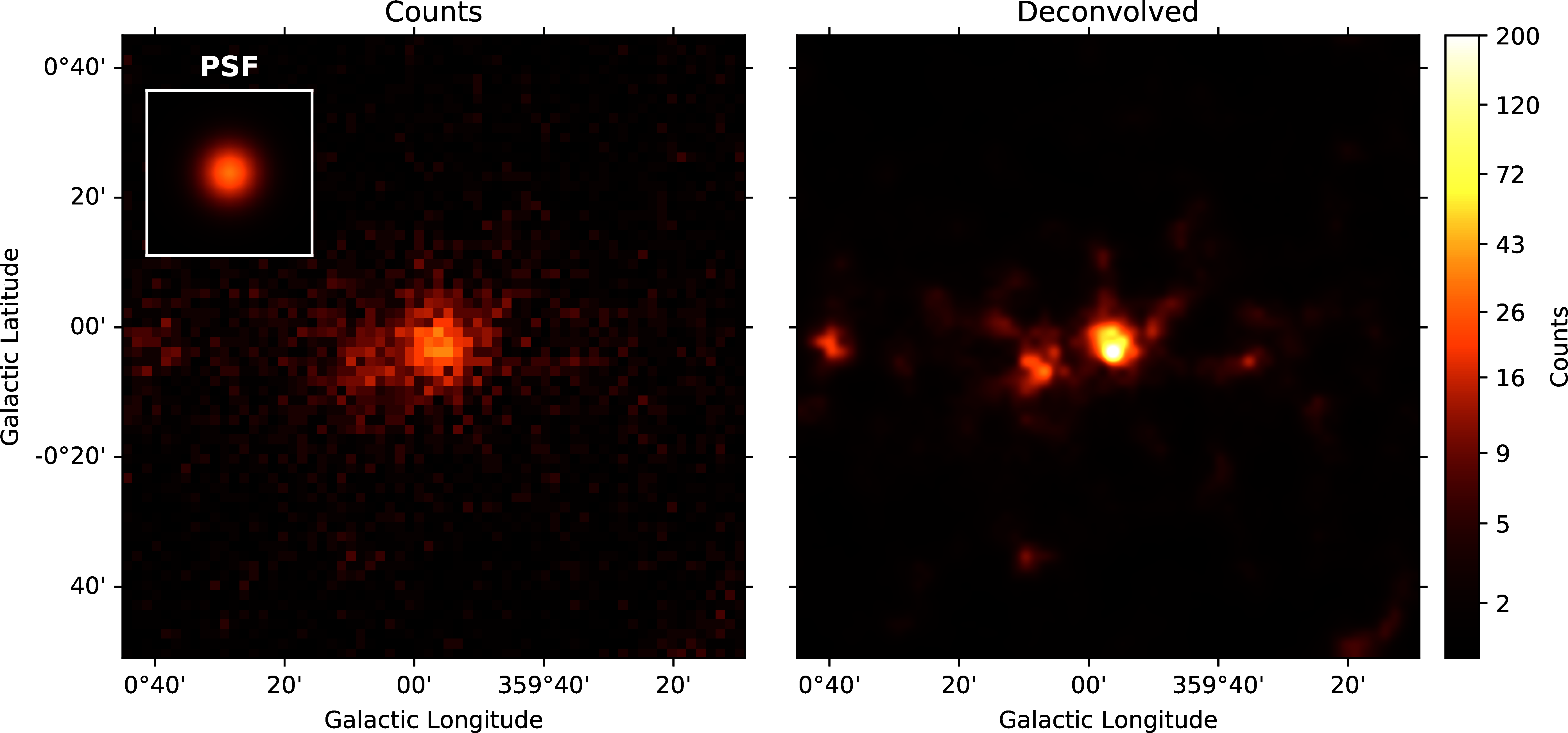
Figure 6:Pylira applied to Fermi-LAT data from the Galactic Center region. The image on the left shows the raw measured counts between 5 and 1000 GeV. The image on the right shows the deconvolved version. The LIRA hyperprior values were chosen as ms_al_kap1=1, ms_al_kap2=0.02, ms_al_kap3=1. No baseline background model was included.
Summary & Outlook
The Pylira package provides Python wrappers for the LIRA algorithm. It allows the deconvolution of low-counts data following Poisson statistics using a Bayesian sampling approach and a multi-scale smoothing prior assumption. The results can be easily written to FITS files and inspected by plotting the trace of the sampling process. This allows users to check for general convergence as well as pixel to pixel correlations for selected regions of interest. The package is openly developed on GitHub and includes tests and documentation, such that it can be maintained and improved in the future, while ensuring consistency of the results. It comes with multiple built-in test datasets and explanatory tutorials in the form of Jupyter notebooks. Future plans include the support for parallelisation or distributed computing, more flexible prior definitions and the possibility to account for systematic errors on the PSF during the sampling process.
This work was conducted under the auspices of the CHASC International Astrostatistics Center. CHASC is supported by NSF grants DMS-21-13615, DMS-21-13397, and DMS-21-13605; by the UK Engineering and Physical Sciences Research Council [EP/W015080/1]; and by NASA 18-APRA18-0019. We thank CHASC members for many helpful discussions, especially Xiao-Li Meng and Katy McKeough. DvD was also supported in part by a Marie-Skodowska-Curie RISE Grant (H2020-MSCA-RISE-2019-873089) provided by the European Commission. Aneta Siemiginowska, Vinay Kashyap, and Doug Burke further acknowledge support from NASA contract to the Chandra X-ray Center NAS8-03060.
Copyright © 2022 Donath et al. This is an open-access article distributed under the terms of the Creative Commons Attribution 3.0 Unported license.
- ACIS
- Advanced CCD Imaging Spectrometer
- HRC
- high-resolution camera
- LAT
- Large Area Telescope
- MAP
- Maximum A-Postori
- PSF
- point spread function
- RL
- Richardson & Lucy
- Hogbom, J. A. (1974). Aperture Synthesis with a Non-Regular Distribution of Interferometer Baselines. Astronomy and Astrophysics Supplement, 15, 417.
- Cash, W. (1979). Parameter estimation in astronomy through application of the likelihood ratio. The Astrophysical Journal, 228, 939–947. 10.1086/156922
- Richardson, W. H. (1972). Bayesian-Based Iterative Method of Image Restoration. Journal of the Optical Society of America (1917-1983), 62(1), 55. 10.1364/josa.62.000055
- Lucy, L. B. (1974). An iterative technique for the rectification of observed distributions. Astronomical Journal, 79, 745. 10.1086/111605
- van der Walt, S., Schönberger, J. L., Nunez-Iglesias, J., Boulogne, F., Warner, J. D., Yager, N., Gouillart, E., Yu, T., & the scikit-image contributors. (2014). scikit-image: image processing in Python. PeerJ, 2, e453. 10.7717/peerj.453
- Hastings, W. K. (1970). Monte Carlo Sampling Methods using Markov Chains and their Applications. Biometrika, 57(1), 97–109. 10.1093/biomet/57.1.97
- Perry, K. M., & Reeves, S. J. (1994). Generalized Cross-Validation as a Stopping Rule for the Richardson-Lucy Algorithm. In R. J. Hanisch & R. L. White (Eds.), The Restoration of HST Images and Spectra - II (p. 97). 10.1002/ima.1850060412
- Fish, D. A., Brinicombe, A. M., Pike, E. R., & Walker, J. G. (1995). Blind deconvolution by means of the Richardson–Lucy algorithm. J. Opt. Soc. Am. A, 12(1), 58–65. 10.1364/JOSAA.12.000058
- Esch, D. N., Connors, A., Karovska, M., & van Dyk, D. A. (2004). An Image Restoration Technique with Error Estimates. The Astrophysical Journal, 610(2), 1213–1227. 10.1086/421761
- Connors, A., Stein, N. M., van Dyk, D., Kashyap, V., & Siemiginowska, A. (2011). LIRA — The Low-Counts Image Restoration and Analysis Package: A Teaching Version via R. In I. N. Evans, A. Accomazzi, D. J. Mink, & A. H. Rots (Eds.), Astronomical Data Analysis Software and Systems XX (Vol. 442, p. 463).
- R Core Team. (2020). R: A Language and Environment for Statistical Computing. R Foundation for Statistical Computing. https://www.R-project.org/
- Jakob, W., Rhinelander, J., & Moldovan, D. (2017). pybind11 – Seamless operability between C++11 and Python.
- Harris, C. R., Millman, K. J., van der Walt, S. J., Gommers, R., Virtanen, P., Cournapeau, D., Wieser, E., Taylor, J., Berg, S., Smith, N. J., Kern, R., Picus, M., Hoyer, S., van Kerkwijk, M. H., Brett, M., Haldane, A., del Río, J. F., Wiebe, M., Peterson, P., … Oliphant, T. E. (2020). Array programming with NumPy. Nature, 585(7825), 357–362. 10.1038/s41586-020-2649-2
- Collaboration, A. (2018). The Astropy Project: Building an Open-science Project and Status of the v2.0 Core Package. The Astrophysical Journal, 156(3), 123. 10.3847/1538-3881/aabc4f
- Hunter, J. D. (2007). Matplotlib: A 2D graphics environment. Computing in Science & Engineering, 9(3), 90–95. 10.1109/MCSE.2007.55
