Incorporating Task-Agnostic Information in Task-Based Active Learning Using a Variational Autoencoder
Abstract
It is often much easier and less expensive to collect data than to label it. Active learning (AL) Settles, 2009 responds to this issue by selecting which unlabeled data are best to label next. Standard approaches utilize task-aware AL, which identifies informative samples based on a trained supervised model. Task-agnostic AL ignores the task model and instead makes selections based on learned properties of the dataset. We seek to combine these approaches and measure the contribution of incorporating task-agnostic information into standard AL, with the suspicion that the extra information in the task-agnostic features may improve the selection process. We test this on various AL methods using a ResNet classifier with and without added unsupervised information from a variational autoencoder (VAE). Although the results do not show a significant improvement, we investigate the effects on the acquisition function and suggest potential approaches for extending the work.
Introduction
In deep learning, the capacity for data gathering often significantly outpaces the labeling. This is easily observed in the field of bioimaging, where ground-truth labeling usually requires the expertise of a clinician. For example, producing a large quantity of CT scans is relatively simple, but having them labeled for COVID-19 by cardiologists takes much more time and money. These constraints ultimately limit the contribution of deep learning to many crucial research problems.
This labeling issue has compelled advancements in the field of active learning (AL) Settles, 2009. In a typical AL setting, there is a set of labeled data and a (usually larger) set of unlabeled data. A model is trained on the labeled data, then the model is analyzed to evaluate which unlabeled points should be labeled to best improve the loss objective after further training. AL acknowledges labeling constraints by specifying a budget of points that can be labeled at a time and evaluating against this budget.
In AL, the model for which we select new labels is referred to as the task model. If this model is a classifier neural network, the space in which it maps inputs before classifying them is known as the latent space or representation space. A recent branch of AL Sener & Savarese, 2018Smailagic et al., 2018Yoo & Kweon, 2019, prominent for its applications to deep models, focuses on mapping unlabeled points into the task model’s latent space before comparing them.
These methods are limited in their analysis by the labeled data they must train on, failing to make use of potentially useful information embedded in the unlabeled data. We therefore suggest that this family of methods may be improved by extending their representation spaces to include unsupervised features learned over the entire dataset. For this purpose, we opt to use a variational autoencoder (VAE) Kingma & Welling, 2013, which is a prominent method for unsupervised representation learning. Our main contributions are (a) a new methodology for extending AL methods using VAE features and (b) an experiment comparing AL performance across two recent feature-based AL methods using the new method.
Related Literature
Active learning
Much of the early active learning (AL) literature is based on shallower, less computationally demanding networks since deeper architectures were not well-developed at the time. Settles (2009) provides a review of these early methods. The modern approach uses an acquisition function, which involves ranking all available unlabeled points by some chosen heuristic and choosing to label the points of highest ranking.
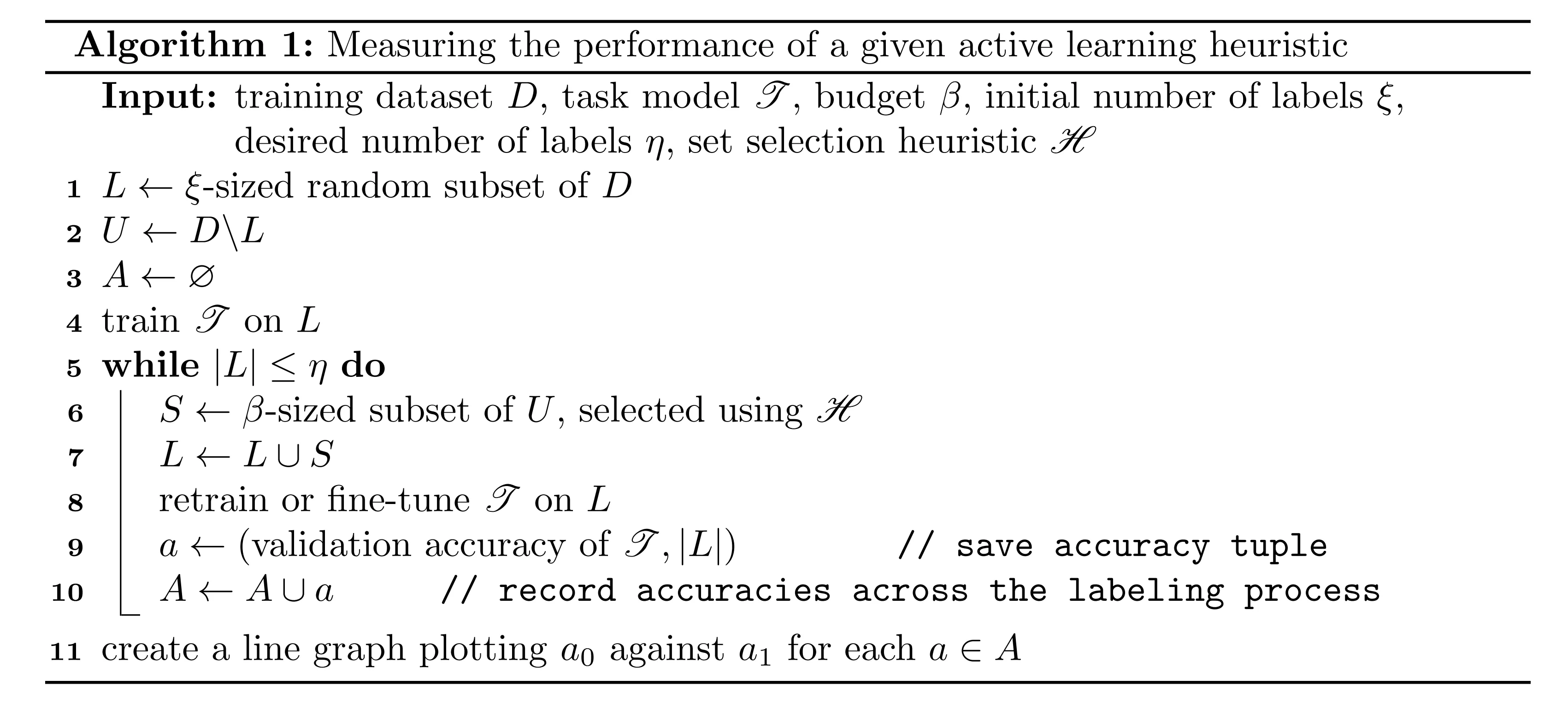
The popularity of the acquisition approach has led to a widely-used evaluation procedure, which we describe in Algorithm 1. This procedure trains a task model on the initial labeled data, records its test accuracy, then uses to label a set of unlabeled points. We then once again train on the labeled data and record its accuracy. This is repeated until a desired number of labels is reached, and then the accuracies can be graphed against the number of available labels to demonstrate performance over the course of labeling. We can use this evaluation algorithm to separately evaluate multiple acquisition functions on their resulting accuracy graphs. This is utilized in many AL papers to show the efficacy of their suggested heuristics in comparison to others Wang et al., 2016Sener & Savarese, 2018Smailagic et al., 2018Yoo & Kweon, 2019.
The prevailing approach to point selection has been to choose unlabeled points for which the model is most uncertain, the assumption being that uncertain points will be the most informative Budd et al., 2021. A popular early method was to label the unlabeled points of highest Shannon entropy Shannon, 1948 under the task model, which is a measure of uncertainty between the classes of the data. This method is now more commonly used in combination with a representativeness measure Wang et al., 2016 to avoid selecting condensed clusters of very similar points.
Recent heuristics using deep features
For convolutional neural networks (CNNs) in image classification settings, the task model can be decomposed into a feature-generating module
which maps the input data vectors to the output of the final fully connected layer before classification, and a classification module
where is the number of classes.
Recent deep learning-based AL methods have approached the notion of model uncertainty in terms of the rich features generated by the learned model. Core-set Sener & Savarese, 2018 and MedAL Smailagic et al., 2018 select unlabeled points that are the furthest from the labeled set in terms of distance between the learned features. For core-set, each point constructing the set in step 6 of Algorithm 1 is chosen by
where is the unlabeled set and is the labeled set. The analogous operation for MedAL is
Note that after a point is chosen, the selection of the next point assumes the previous to be in the labeled set. This way we discourage choosing sets that are closely packed together, leading to sets that are more diverse in terms of their features. This effect is more pronounced in the core-set method since it takes the minimum distance whereas MedAL uses the average distance.
Another recent method Yoo & Kweon, 2019 trains a regression network to predict the loss of the task model, then takes the heuristic in Algorithm 1 to select the unlabeled points of highest predicted loss. To implement this, the loss prediction network is attached to a ResNet task model and is trained jointly with . The inputs to are the features output by the ResNet’s four residual blocks. These features are mapped into the same dimensionality via a fully connected layer and then concatenated to form a representation . An additional fully connected layer then maps into a single value constituting the loss prediction.
When attempting to train a network to directly predict ’s loss during training, the ground truth losses naturally decrease as is optimized, resulting in a moving objective. The authors of Yoo & Kweon (2019) find that a more stable ground truth is the inequality between the losses of given pairs of points. In this case, is trained on pairs of labeled points, so that is penalized for producing predicted loss pairs that exhibit a different inequality than the corresponding true loss pair.
More specifically, for each batch of labeled data that is propagated through during training, the batch of true losses is computed and split randomly into a batch of pairs . The loss prediction network produces a corresponding batch of predicted loss pairs, denoted . The following pair loss is then computed given each and its corresponding :
where is the following indicator function for pair inequality:
Variational Autoencoders
Variational autoencoders (VAEs) Kingma & Welling, 2013 are an unsupervised method for modeling data using Bayesian posterior inference. We begin with the Bayesian assumption that the data is well-modeled by some distribution, often a multivariate Gaussian. We also assume that this data distribution can be inferred reasonably well by a lower dimensional random variable, also often modeled by a multivariate Gaussian.
The inference process then consists of an encoding into the lower dimensional latent variable, followed by a decoding back into the data dimension. We parametrize both the encoder and the decoder as neural networks, jointly optimizing their parameters with the following loss function Kingma & Welling, 2019:
where θ and ϕ are the parameters of the encoder and the decoder, respectively. The first term is the reconstruction error, penalizing the parameters for producing poor reconstructions of the input data. The second term is the regularization error, encouraging the encoding to resemble a pre-selected prior distribution, commonly a unit Gaussian prior.
The encoder of a well-optimized VAE can be used to generate latent encodings with rich features which are sufficient to approximately reconstruct the data. The features also have some geometric consistency, in the sense that the encoder is encouraged to generate encodings in the pattern of a Gaussian distribution.
Methods
We observe that the notions of uncertainty developed in the core-set and MedAL methods rely on distances between feature vectors modeled by the task model . Additionally, loss prediction relies on a fully connected layer mapping from a feature space to a single value, producing different predictions depending on the values of the relevant feature vector. Thus all of these methods utilize spatial reasoning in a vector space.
Furthermore, in each of these methods, the heuristic only has access to information learned by the task model, which is trained only on the labeled points at a given timestep in the labeling procedure. Since variational autoencoder (VAE) encodings are not limited by the contents of the labeled set, we suggest that the aforementioned methods may benefit by expanding the vector spaces they investigate to include VAE features learned across the entire dataset, including the unlabeled data. These additional features will constitute representative and previously inaccessible information regarding the data, which may improve the active learning process.
We implement this by first training a VAE model on the given dataset. can then be used as a function returning the VAE features for any given datapoint. We append these additional features to the relevant vector spaces using vector concatenation, an operation we denote with the symbol . The modified point selection operation in core-set then becomes
where α is a hyperparameter that scales the influence of the VAE features in computing the vector distance. To similarly modify the loss prediction method, we concatenate the VAE features to the final ResNet feature concatenation before the loss prediction, so that the extra information is factored into the training of the prediction network .
Experiments
In order to measure the efficacy of the newly proposed methods, we generate accuracy graphs using Algorithm 1, freezing all settings except the selection heuristic . We then compare the performance of the core-set and loss prediction heuristics with their VAE-augmented counterparts.
We use ResNet-18 pretrained on ImageNet as the task model, using the SGD optimizer with learning rate 0.001 and momentum 0.9. We train on the MNIST Deng, 2012 and ChestMNIST Yang et al., 2021 datasets. ChestMNIST consists of 112,120 chest X-ray images resized to 28x28 and is one of several benchmark medical image datasets introduced in Yang et al. (2021).
For both datasets we experiment on randomly selected subsets, using 25000 points for MNIST and 30000 points for ChestMNIST. In both cases we begin with 3000 initial labels and label 3000 points per active learning step. We opt to retrain the task model after each labeling step instead of fine-tuning.
We use a similar training strategy as in Smailagic et al. (2018), training the task model until >99% train accuracy before selecting new points to label. This ensures that the ResNet is similarly well fit to the labeled data at each labeling iteration. This is implemented by training for 10 epochs on the initial training set and increasing the training epochs by 5 after each labeling iteration.
The VAEs used for the experiments are trained for 20 epochs using an Adam optimizer with learning rate 0.001 and weight decay 0.005. The VAE encoder architecture consists of four convolutional downsampling filters and two linear layers to learn the low dimensional mean and log variance. The decoder consists of an upsampling convolution and four size-preserving convolutions to learn the reconstruction.
Experiments were run five times, each with a separate set of randomly chosen initial labels, with the displayed results showing the average validation accuracies across all runs. Figure 1 and Figure 3 show the core-set results, while Figure 2 and Figure 4 show the loss prediction results. In all cases, shared random seeds were used to ensure that the task models being compared were supplied with the same initial set of labels.
With four NVIDIA 2080 GPUs, the total runtime for the MNIST experiments was 5113s for core-set and 4955s for loss prediction; for ChestMNIST, the total runtime was 7085s for core-set and 7209s for loss prediction.

Figure 1:The average MNIST results using the core-set heuristic versus the VAE-augmented core-set heuristic for Algorithm 1 over 5 runs.

Figure 2:The average MNIST results using the loss prediction heuristic versus the VAE-augmented loss prediction heuristic for Algorithm 1 over 5 runs.

Figure 3:The average ChestMNIST results using the core-set heuristic versus the VAE-augmented core-set heuristic for Algorithm 1 over 5 runs.

Figure 4:The average ChestMNIST results using the loss prediction heuristic versus the VAE-augmented loss prediction heuristic for Algorithm 1 over 5 runs.
To investigate the qualitative difference between the VAE and non-VAE approaches, we performed an additional experiment to visualize an example of core-set selection. We first train the ResNet-18 with the same hyperparameter settings on 1000 initial labels from the ChestMNIST dataset, then randomly choose 1556 (5%) of the unlabeled points from which to select 100 points to label. These smaller sizes were chosen to promote visual clarity in the output graphs.
We use t-SNE Maaten & Hinton, 2008 dimensionality reduction to show the ResNet features of the labeled set, the unlabeled set, and the points chosen to be labeled by core-set.
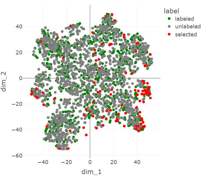
Figure 5:A t-SNE visualization of the ChestMNIST points chosen by core-set.

Figure 6:A t-SNE visualization of the ChestMNIST points chosen by core-set when the ResNet features are augmented with VAE features.
Discussion
Overall, the VAE-augmented active learning heuristics did not exhibit a significant performance difference when compared with their counterparts. The only case of a significant p-value (<0.05) occurred during loss prediction on the MNIST dataset at 21000 labels.
The t-SNE visualizations in Figure 5 and Figure 6 show some of the influence that the VAE features have on the core-set selection process. In Figure 5, the selected points tend to be more spread out, while in Figure 6 they cluster at one edge. This appears to mirror the transformation of the rest of the data, which is more spread out without the VAE features, but becomes condensed in the center when they are introduced, approaching the shape of a Gaussian distribution.
It seems that with the added VAE features, the selected points are further out of distribution in the latent space. This makes sense because points tend to be more sparse at the tails of a Guassian distribution and core-set prioritizes points that are well-isolated from other points.
One reason for the lack of performance improvement may be the homogeneous nature of the VAE, where the optimization goal is reconstruction rather than classification. This could be improved by using a multimodal prior in the VAE, which may do a better job of modeling relevant differences between points.
Conclusion
Our original intuition was that additional unsupervised information may improve established active learning methods, especially when using a modern unsupervised representation method such as a VAE. The experimental results did not indicate this hypothesis, but additional investigation of the VAE features showed a notable change in the task model latent space. Though this did not result in superior point selections in our case, it is of interest whether different approaches to latent space augmentation in active learning may fare better.
Future work may explore the use of class-conditional VAEs in a similar application, since a VAE that can utilize the available class labels may produce more effective representations, and it could be retrained along with the task model after each labeling iteration.
Copyright © 2022 Godwin et al. This is an open-access article distributed under the terms of the Creative Commons Attribution 3.0 Unported license.
- AL
- active learning
- CNN
- convolutional neural network
- VAE
- variational autoencoder
- Settles, B. (2009). Active learning literature survey.
- Sener, O., & Savarese, S. (2018). Active Learning for Convolutional Neural Networks: A Core-Set Approach. International Conference on Learning Representations. https://openreview.net/forum?id=H1aIuk-RW
- Smailagic, A., Costa, P., Noh, H. Y., Walawalkar, D., Khandelwal, K., Galdran, A., Mirshekari, M., Fagert, J., Xu, S., Zhang, P., & others. (2018). Medal: Accurate and robust deep active learning for medical image analysis. 2018 17th IEEE International Conference on Machine Learning and Applications (ICMLA), 481–488. 10.1109/icmla.2018.00078
- Yoo, D., & Kweon, I. S. (2019). Learning loss for active learning. Proceedings of the IEEE/CVF Conference on Computer Vision and Pattern Recognition, 93–102. 10.1109/CVPR.2019.00018
- Kingma, D. P., & Welling, M. (2013). Auto-encoding variational bayes. arXiv Preprint arXiv:1312.6114.
- Wang, K., Zhang, D., Li, Y., Zhang, R., & Lin, L. (2016). Cost-effective active learning for deep image classification. IEEE Transactions on Circuits and Systems for Video Technology, 27(12), 2591–2600. 10.1109/tcsvt.2016.2589879
- Budd, S., Robinson, E. C., & Kainz, B. (2021). A survey on active learning and human-in-the-loop deep learning for medical image analysis. Medical Image Analysis, 71, 102062. 10.1016/j.media.2021.102062
- Shannon, C. E. (1948). A mathematical theory of communication. The Bell System Technical Journal, 27(3), 379–423.
- Kingma, D. P., & Welling, M. (2019). An Introduction to Variational Autoencoders. Now Publishers. 10.1561/9781680836233
- Deng, L. (2012). The mnist database of handwritten digit images for machine learning research. IEEE Signal Processing Magazine, 29(6), 141–142. 10.1109/MSP.2012.2211477
- Yang, J., Shi, R., & Ni, B. (2021). MedMNIST Classification Decathlon: A Lightweight AutoML Benchmark for Medical Image Analysis. 2021 IEEE 18th International Symposium on Biomedical Imaging (ISBI), 191–195. 10.1109/ISBI48211.2021.9434062
- Van der Maaten, L., & Hinton, G. (2008). Visualizing data using t-SNE. Journal of Machine Learning Research, 9(11).