
poliastro: a Python library for interactive astrodynamics
Abstract
Space is more popular than ever, with the growing public awareness of interplanetary scientific missions, as well as the increasingly large number of satellite companies planning to deploy satellite constellations. Python has become a fundamental technology in the astronomical sciences, and it has also caught the attention of the Space Engineering community.
One of the requirements for designing a space mission is studying the trajectories of satellites, probes, and other artificial objects, usually ignoring non-gravitational forces or treating them as perturbations: the so-called n-body problem. However, for preliminary design studies and most practical purposes, it is sufficient to consider only two bodies: the object under study and its attractor.
Even though the two-body problem has many analytical solutions, orbit propagation (the initial value problem) and targeting (the boundary value problem) remain computationally intensive because of long propagation times, tight tolerances, and vast solution spaces. On the other hand, astrodynamics researchers often do not share the source code they used to run analyses and simulations, which makes it challenging to try out new solutions.
This paper presents poliastro, an open-source Python library for interactive astrodynamics that features an easy-to-use API and tools for quick visualization. poliastro implements core astrodynamics algorithms (such as the resolution of the Kepler and Lambert problems) and leverages numba, a Just-in-Time compiler for scientific Python, to optimize the running time. Thanks to Astropy, poliastro can perform seamless coordinate frame conversions and use proper physical units and timescales. At the moment, poliastro is the longest-lived Python library for astrodynamics, has contributors from all around the world, and several New Space companies and people in academia use it.
Introduction
History
The term “astrodynamics” was coined by the American astronomer Samuel Herrick, who received encouragement from the space pioneer Robert H. Goddard, and refers to the branch of space science dealing with the motion of artificial celestial bodies Duboshin, 1973Herrick, 1971. However, the roots of its mathematical foundations go back several centuries.
Kepler first introduced his laws of planetary motion in 1609 and 1619 and derived his famous transcendental equation (1), which we now see as capturing a restricted form of the two-body problem. This work was generalized by Newton to give birth to the n-body problem, and many other mathematicians worked on it throughout the centuries (Daniel and Johann Bernoulli, Euler, Gauss). Poincaré established in the 1890s that no general closed-form solution exists for the n-body problem, since the resulting dynamical system is chaotic Battin, 1999. Sundman proved in the 1900s the existence of convergent solutions for a few restricted with .
In 1903 Tsiokovsky evaluated the conditions required for artificial objects to leave the orbit of the earth; this is considered as a foundational contribution to the field of astrodynamics. Tsiokovsky devised equation (2) which relates the increase in velocity with the effective exhaust velocity of thrusted gases and the fraction of used propellant.
Further developments by Kondratyuk, Hohmann, and Oberth in the early 20th century all added to the growing field of orbital mechanics, which in turn enabled the development of space flight in the USSR and the United States in the 1950s and 1960s.
The two-body problem
In a system of bodies subject to their mutual attraction, by application of Newton’s law of universal gravitation, the total force affecting due to the presence of the other masses is given by Battin (1999):
where is the universal gravitational constant, and denotes the position vector from to . Applying Newton’s second law of motion results in a system of differential equations:
By setting in (4) and subtracting the two resulting equalities, one arrives to the fundamental equation of the two-body problem:
where . When (for example, an artificial satellite orbiting a planet), one can consider a property of the attractor.
Keplerian vs non-keplerian motion
Conveniently manipulating equation (5) leads to several properties Battin, 1999 that were already published by Johannes Kepler in the 1610s, namely:
- The orbit always describes a conic section (an ellipse, a parabola, or an hyperbola), with the attractor at one of the two foci and can be written in polar coordinates like (Kepler’s first law).
- The magnitude of the specific angular momentum is constant an equal to two times the areal velocity (Kepler’s second law).
- For closed (circular and elliptical) orbits, the period is related to the size of the orbit through (Kepler’s third law).
For many practical purposes it is usually sufficient to limit the study to one object orbiting an attractor and ignore all other external forces of the system, hence restricting the study to trajectories governed by equation (5). Such trajectories are called “Keplerian”, and several problems can be formulated for them:
- The initial-value problem, which is usually called propagation, involves determining the position and velocity of an object after an elapse period of time given some initial conditions.
- Preliminary orbit determination, which involves using exact or approximate methods to derive a Keplerian orbit from a set of observations.
- The boundary-value problem, often named the Lambert problem, which involves determining a Keplerian orbit from boundary conditions, usually departure and arrival position vectors and a time of flight.
Fortunately, most of these problems boil down to finding numerical solutions to relatively simple algebraic relations between time and angular variables: for elliptic motion () it is the Kepler equation, and equivalent relations exist for the other eccentricity regimes Battin, 1999. Numerical solutions for these equations can be found in a number of different ways, each one with different complexity and precision tradeoffs. In the Methods section we list the ones implemented by poliastro.
On the other hand, there are many situations in which natural and artificial orbital perturbations must be taken into account so that the actual non-Keplerian motion can be properly analyzed:
- Interplanetary travel in the proximity of other planets. On a first approximation it is usually enough to study the trajectory in segments and focus the analysis on the closest attractor, hence patching several Keplerian orbits along the way (the so-called “patched-conic approximation”) Battin, 1999. The boundary surface that separates one segment from the other is called the sphere of influence.
- Use of solar sails, electric propulsion, or other means of continuous thrust. Devising the optimal guidance laws that minimize travel time or fuel consumption under these conditions is usually treated as an optimization problem of a dynamical system, and as such it is particularly challenging Conway, 2014.
- Artificial satellites in the vicinity of a planet. This is the regime in which all the commercial space industry operates, especially for those satellites in Low-Earth Orbit (LEO).
State of the art
In our view, at the time of creating poliastro there were a number of issues with existing open source astrodynamics software that posed a barrier of entry for novices and amateur practitioners. Most of these barriers still exist today and are described in the following paragraphs. The goals of the project can be condensed as follows:
- Set an example on reproducibility and good coding practices in astrodynamics.
- Become an approachable software even for novices.
- Offer a performant software that can be also used in scripting and interactive workflows.
The most mature software libraries for astrodynamics are arguably Orekit Orekit, 2022, a “low level space dynamics library written in Java” with an open governance model, and SPICE SPICE, 2022, a toolkit developed by NASA’s Navigation and Ancillary Information Facility at the Jet Propulsion Laboratory. Other similar, smaller projects that appeared later on and that are still maintained to this day include PyKEP Izzo et al., 2020, beyond beyond, 2022, tudatpy tudatpy, 2022, sbpy Mommert et al., 2019, Skyfield Rhodes, 2020 (Python), CelestLab (Scilab) celestlab, 2022, astrodynamics.jl (Julia) Astrodynamics.jl, n.d. and Nyx (Rust) nyx, 2021. In addition, there are some Graphical User Interface (GUI) based open source programs used for Mission Analysis and orbit visualization, such as GMAT GMAT, 2020 and gpredict gpredict, 2018, and complete web applications for tracking constellations of satellites like the SatNOGS project by the Libre Space Foundation SatNOGS, 2021.
The level of quality and maintenance of these packages is somewhat heterogeneous. Community-led projects with a strong corporate backing like Orekit are in excellent health, while on the other hand smaller projects developed by volunteers (beyond, astrodynamics.jl) or with limited institutional support (PyKEP, GMAT) suffer from lack of maintenance. Part of the problem might stem from the fact that most scientists are never taught how to build software efficiently, let alone the skills to collaboratively develop software in the open Wilson et al., 2014, and astrodynamicists are no exception.
On the other hand, it is often difficult to translate the advances in astrodynamics research to software. Classical algorithms developed throughout the 20th century are described in papers that are sometimes difficult to find, and source code or validation data is almost never available. When it comes to modern research carried in the digital era, source code and validation data is still difficult, even though they are supposedly provided “upon reasonable request” Stodden et al., 2018Gabelica et al., 2022.
It is no surprise that astrodynamics software often requires deep expertise. However, there are often implicit assumptions that are not documented with an adequate level of detail which originate widespread misconceptions and lead even seasoned professionals to make conceptual mistakes. Some of the most notorious misconceptions arise around the use of general perturbations data (OMMs and TLEs) Finkleman, 2007, the geometric interpretation of the mean anomaly Battin, 1999, or coordinate transformations Vallado et al., 2006.
Finally, few of the open source software libraries mentioned above are amenable to scripting or interactive use, as promoted by computational notebooks like Jupyter Kluyver et al., 2016.
The following sections will now discuss the various areas of current research that an astrodynamicist will engage in, and how poliastro improves their workflow.
Methods
Software Architecture
The architecture of poliastro emerges from the following set of conflicting requirements:
- There should be a high-level API that enables users to perform orbital calculations in a straightforward way and prevent typical mistakes.
- The running time of the algorithms should be within the same order of magnitude of existing compiled implementations.
- The library should be written in a popular open-source language to maximize adoption and lower the barrier to external contributors.
One of the most typical mistakes we set ourselves to prevent with the high-level API is dimensional errors. Addition and substraction operations of physical quantities are defined only for quantities with the same units Drobot, 1953: for example, the operation requires a scale transformation of at least one of the operands, since they have different units (kilometers and meters) but the same dimension (length), whereas the operation is directly not allowed because dimensions are incompatible (length and mass). As such, software systems operating with physical quantities should raise exceptions when adding different dimensions, and transparently perform the required scale transformations when adding different units of the same dimension.
With this in mind, we evaluated several Python packages for unit handling
(see J. Goldbaum et al. (2018) for a recent survey) and chose astropy.units
The Astropy Collaboration et al., 2018.
radius = 6000  # km
altitude = 500  # m

# Wrong!
distance = radius + altitude

from astropy import units as u

# Correct
distance = (radius << u.km) + (altitude << u.m)
This notion of providing a “safe” API extends to other parts of the library
by leveraging other capabilities of the Astropy project.
For example, timestamps use astropy.time objects,
which take care of the appropriate handling of time scales (such as TDB or UTC),
reference frame conversions leverage astropy.coordinates, and so forth.
One of the drawbacks of existing unit packages is that
they impose a significant performance penalty.
Even though astropy.units is integrated with NumPy,
hence allowing the creation of array quantities,
all the unit compatibility checks are implemented in Python
and require lots of introspection,
and this can slow down mathematical operations by several orders of magnitude.
As such, to fulfill our desired performance requirement for poliastro,
we envisioned a two-layer architecture:
- The Core API follows a procedural style, and all the functions receive Python numerical types and NumPy arrays for maximum performance.
- The High level API is object-oriented, all the methods
receive Astropy
Quantityobjects with physical units, and computations are deferred to the Core API.
Most of the methods of the High level API consist only of the necessary unit compatibility checks, plus a wrapper over the corresponding Core API function that performs the actual computation.
@u.quantity_input(E=u.rad, ecc=u.one)
def E_to_nu(E, ecc):
    """True anomaly from eccentric anomaly."""
    return (
        E_to_nu_fast(
            E.to_value(u.rad),
            ecc.value
        ) << u.rad
    ).to(E.unit)
As a result, poliastro offers a unit-safe API that performs the least amount of computation possible to minimize the performance penalty of unit checks, and also a unit-unsafe API that offers maximum performance at the cost of not performing any unit validation checks.

Figure 1:poliastro two-layer architecture
Finally, there are several options to write performant code that can be used from Python, and one of them is using a fast, compiled language for the CPU intensive parts. Successful examples of this include NumPy, written in C Harris et al., 2020, SciPy, featuring a mix of FORTRAN, C, and C++ code Virtanen et al., 2020, and pandas, making heavy use of Cython Behnel et al., 2011. However, having to write code in two different languages hinders the development speed, makes debugging more difficult, and narrows the potential contributor base (what Julia creators called “The Two Language Problem” Bezanson et al., 2017).
As authors of poliastro we wanted to use Python as the sole programming language of the implementation, and the best solution we found to improve its performance was to use Numba, a LLVM-based Python JIT compiler Lam et al., 2015.
Usage
Basic Orbit and Ephem creation
The two central objects of the poliastro high level API are Orbit and Ephem:
Orbitobjects represent an osculating (hence Keplerian) orbit of a dimensionless object around an attractor at a given point in time and a certain reference frame.Ephemobjects represent an ephemerides, a sequence of spatial coordinates over a period of time in a certain reference frame.
There are six parameters that uniquely determine a Keplerian orbit, plus the gravitational parameter of the corresponding attractor ( or μ). Optionally, an epoch that contextualizes the orbit can be included as well. This set of six parameters is not unique, and several of them have been developed over the years to serve different purposes. The most widely used ones are:
- Cartesian elements: Three components for the position and three components for the velocity . This set has no singularities.
- Classical Keplerian elements: Two components for the shape of the conic (usually the semimajor axis or semiparameter and the eccentricity ), three Euler angles for the orientation of the orbital plane in space (inclination , right ascension of the ascending node Ω, and argument of periapsis ω), and one polar angle for the position of the body along the conic (usually true anomaly or ν). This set of elements has an easy geometrical interpretation and the advantage that, in pure two-body motion, five of them are fixed and only one is time-dependent (ν), which greatly simplifies the analytical treatment of orbital perturbations. However, they suffer from singularities steming from the Euler angles (“gimbal lock”) and equations expressed in them are ill-conditioned near such singularities.
- Walker modified equinoctial elements: Six parameters . Only is time-dependent and this set has no singularities, however the geometrical interpretation of the rest of the elements is lost Walker et al., 1985.
Here is how to create an Orbit from cartesian and from classical Keplerian elements.
Walker modified equinoctial elements are supported as well.
from astropy import units as u

from poliastro.bodies import Earth, Sun
from poliastro.twobody import Orbit
from poliastro.constants import J2000

# Data from Curtis, example 4.3
r = [-6045, -3490, 2500] << u.km
v = [-3.457, 6.618, 2.533] << u.km / u.s

orb_curtis = Orbit.from_vectors(
   Earth,  # Attractor
   r, v  # Elements
)

# Data for Mars at J2000 from JPL HORIZONS
a = 1.523679 << u.au
ecc = 0.093315 << u.one
inc = 1.85 << u.deg
raan = 49.562 << u.deg
argp = 286.537 << u.deg
nu = 23.33 << u.deg

orb_mars = Orbit.from_classical(
   Sun,
   a, ecc, inc, raan, argp, nu,
   J2000  # Epoch
)
When displayed on an interactive REPL, Orbit objects
provide basic information about the geometry, the attractor, and the epoch:
>>> orb_curtis
7283 x 10293 km x 153.2 deg (GCRS) orbit
around Earth (X) at epoch J2000.000 (TT)

>>> orb_mars
1 x 2 AU x 1.9 deg (HCRS) orbit
around Sun (X) at epoch J2000.000 (TT)
Similarly, Ephem objects can be created using a variety of classmethods as well.
Thanks to astropy.coordinates built-in low-fidelity ephemerides,
as well as its capability to remotely access the JPL HORIZONS system,
the user can seamlessly build an object that contains the time history
of the position of any Solar System body:
from astropy.time import Time
from astropy.coordinates import solar_system_ephemeris

from poliastro.ephem import Ephem

# Configure high fidelity ephemerides globally
# (requires network access)
solar_system_ephemeris.set("jpl")

# For predefined poliastro attractors
earth = Ephem.from_body(Earth, Time.now().tdb)

# For the rest of the Solar System bodies
ceres = Ephem.from_horizons("Ceres", Time.now().tdb)
There are some crucial differences between Orbit and Ephem objects:
Orbitobjects have an attractor, whereasEphemobjects do not. Ephemerides can originate from complex trajectories that don’t necessarily conform to the ideal two-body problem.Orbitobjects capture a precise instant in a two-body motion plus the necessary information to propagate it forward in time indefinitely, whereasEphemobjects represent a bounded time history of a trajectory. This is because the equations for the two-body motion are known, whereas an ephemeris is either an observation or a prediction that cannot be extrapolated in any case without external knowledge. As such,Orbitobjects have a.propagatemethod, butEphemones do not. This prevents users from attempting to propagate the position of the planets, which will always yield poor results compared to the excellent ephemerides calculated by external entities.
Finally, both types have methods to convert between them:
Ephem.from_orbitis the equivalent of sampling a two-body motion over a given time interval. As explained above, the resultingEphemloses the information about the original attractor.Orbit.from_ephemis the equivalent of calculating the osculating orbit at a certain point of a trajectory, assuming a given attractor. The resultingOrbitloses the information about the original, potentially complex trajectory.
Orbit propagation
Orbit objects have a .propagate method that takes an elapsed time
and returns another Orbit with new orbital elements and an updated epoch:
>>> from poliastro.examples import iss

>>> iss
>>> 6772 x 6790 km x 51.6 deg (GCRS) ...

>>> iss.nu.to(u.deg)
<Quantity 46.59580468 deg>

>>> iss_30m = iss.propagate(30 << u.min)

>>> (iss_30m.epoch - iss.epoch).datetime
datetime.timedelta(seconds=1800)

>>> (iss_30m.nu - iss.nu).to(u.deg)
<Quantity 116.54513153 deg>
The default propagation algorithm is an analytical procedure described in Farnocchia et al. (2013) that works seamlessly in the near parabolic region. In addition, poliastro implements analytical propagation algorithms as described in Danby & Burkardt (1983)Odell & Gooding (1986)Markley (1995)Mikkola (1987)Pimienta-Penalver (2013)Charls (2022)Vallado & McClain (2007).
Natural perturbations

Figure 2:Osculating (Keplerian) vs perturbed (true) orbit (source: Wikipedia, CC BY-SA 3.0)
As showcased in Figure 2, at any point in a trajectory we can define an ideal Keplerian orbit with the same position and velocity under the attraction of a point mass: this is called the osculating orbit. Some numerical propagation methods exist that model the true, perturbed orbit as a deviation from an evolving, osculating orbit. poliastro implements Cowell’s method Cowell & Crommelin, 1910, which consists in adding all the perturbation accelerations and then integrating the resulting differential equation with any numerical method of choice:
The resulting equation is usually integrated using high order numerical methods,
since the integration times are quite large and the tolerances comparatively tight.
An in-depth discussion of such methods can be found in Hairer et al. (2009).
poliastro uses Dormand-Prince 8(5,3) (DOP853), a commonly used method
available in SciPy Harris et al., 2020.
There are several natural perturbations included: J2 and J3 gravitational terms, several atmospheric drag models (exponential, Jacchia (1977), Atmosphere et al. (1962), Atmosphere et al. (1976)), and helpers for third body gravitational attraction and radiation pressure as described in Curtis (2010).
@njit
def combined_a_d(
    t0, state, k, j2, r_eq, c_d, a_over_m, h0, rho0
):
    return (
        J2_perturbation(
            t0, state, k, j2, r_eq
        ) + atmospheric_drag_exponential(
            t0, state, k, r_eq, c_d, a_over_m, h0, rho0
        )
    )

def f(t0, state, k):
    du_kep = func_twobody(t0, state, k)
    ax, ay, az = combined_a_d(
        t0,
        state,
        k,
        R=R,
        C_D=C_D,
        A_over_m=A_over_m,
        H0=H0,
        rho0=rho0,
        J2=Earth.J2.value,
    )
    du_ad = np.array([0, 0, 0, ax, ay, az])

    return du_kep + du_ad

rr = propagate(
    orbit,
    tofs,
    method=cowell,
    f=f,
)
Continuous thrust control laws
Beyond natural perturbations, spacecraft can modify their trajectory on purpose by using impulsive maneuvers (as explained in the next section) as well as continuous thrust guidance laws. The user can define custom guidance laws by providing a perturbation acceleration in the same way natural perturbations are used. In addition, poliastro includes several analytical solutions for continuous thrust guidance laws with specific purposes, as studied in Cano Rodríguez (2017): optimal transfer between circular coplanar orbits Edelbaum, 1961Burt, 1967, optimal transfer between circular inclined orbits Edelbaum, 1961Kechichian, 1997, quasi-optimal eccentricity-only change Pollard, 1997, simultaneous eccentricity and inclination change Pollard, 2000, and agument of periapsis adjustment Pollard, 1998. A much more rigorous analysis of a similar set of laws can be found in Di Carlo & Vasile (2021).
from poliastro.twobody.thrust import change_ecc_inc

ecc_f = 0.0 << u.one
inc_f = 20.0 << u.deg
f = 2.4e-6 << (u.km / u.s**2)

a_d, _, t_f = change_ecc_inc(orbit, ecc_f, inc_f, f)
Impulsive maneuvers
Impulsive maneuvers are modeled considering a change in the velocity of a
spacecraft while its position remains fixed. The poliastro.maneuver.Maneuver
class provides various constructors to instantiate popular impulsive maneuvers
in the framework of the non-perturbed two-body problem:
Maneuver.impulseManeuver.hohmannManeuver.biellipticManeuver.lambert
from poliastro.maneuver import Maneuver

orb_i = Orbit.circular(Earth, alt=700 << u.km)
hoh = Maneuver.hohmann(orb_i, r_f=36000 << u.km)
Once instantiated, Maneuver objects provide information regarding total
and :
>>> hoh.get_total_cost()
<Quantity 3.6173981270031357 km / s>

>>> hoh.get_total_time()
<Quantity 15729.741535747102 s>
Maneuver objects can be applied to Orbit instances using the
apply_maneuver method.
>>> orb_i
7078 x 7078 km x 0.0 deg (GCRS) orbit
around Earth (X)

>>> orb_f = orb_i.apply_maneuver(hoh)
>>> orb_f
36000 x 36000 km x 0.0 deg (GCRS) orbit
around Earth (X)
Targeting
Targeting is the problem of finding the orbit connecting two positions over a finite amount of time. Within the context of the non-perturbed two-body problem, targeting is just a matter of solving the BVP, also known as Lambert’s problem. Because targeting tries to find for an orbit, the problem is included in the Initial Orbit Determination field.
The poliastro.iod package contains izzo and vallado modules. These
provide a lambert function for solving the targeting problem. Nevertheless,
a Maneuver.lambert constructor is also provided so users can keep taking
advantage of Orbit objects.
# Declare departure and arrival datetimes
date_launch = time.Time(
    '2011-11-26 15:02', scale='tdb'
)
date_arrival = time.Time(
    '2012-08-06 05:17', scale='tdb'
)

# Define initial and final orbits
orb_earth = Orbit.from_ephem(
    Sun, Ephem.from_body(Earth, date_launch),
    date_launch
)
orb_mars = Orbit.from_ephem(
    Sun, Ephem.from_body(Mars, date_arrival),
    date_arrival
)

# Compute targetting maneuver and apply it
man_lambert = Maneuver.lambert(orb_earth, orb_mars)
orb_trans, orb_target = ss0.apply_maneuver(
    man_lambert, intermediate=true
)
Targeting is closely related to quick mission design by means of porkchop diagrams. These are contour plots showing all combinations of departure and arrival dates with the specific energy for each transfer orbit. They allow for quick identification of the most optimal transfer dates between two bodies.
The poliastro.plotting.porkchop provides the PorkchopPlotter class which
allows the user to generate these diagrams.
from poliastro.plotting.porkchop import (
    PorkchopPlotter
)
from poliastro.utils import time_range

# Generate all launch and arrival dates
launch_span = time_range(
    "2020-03-01", end="2020-10-01", periods=int(150)
)
arrival_span = time_range(
    "2020-10-01", end="2021-05-01", periods=int(150)
)

# Create an instance of the porkchop and plot it
porkchop = PorkchopPlotter(
    Earth, Mars, launch_span, arrival_span,
)
Previous code, with some additional customization, generates Figure 3.
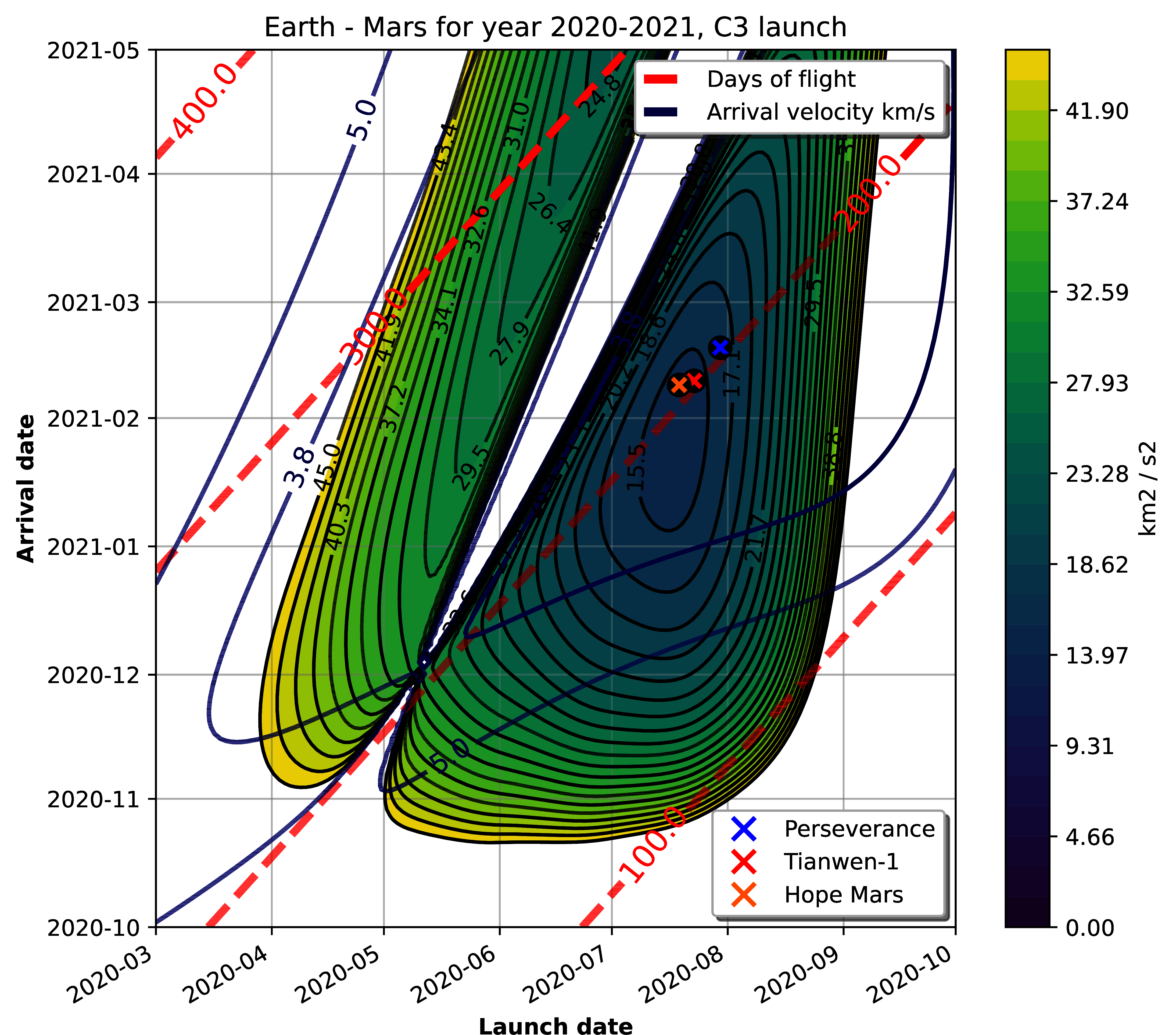
Figure 3:Porkchop plot for Earth-Mars transfer arrival energy showing latest missions to the Martian planet.
Plotting
For visualization purposes, poliastro provides the poliastro.plotting
package, which contains various utilities for generating 2D and 3D graphics
using different backends such as matplotlib Hunter, 2007 and Plotly Plotly Technologies Inc., 2015.
Generated graphics can be static or interactive. The main difference between these two is the ability to modify the camera view in a dynamic way when using interactive plotters.
The most important classes in the poliastro.plotting package are
StaticOrbitPlotter and OrbitPlotter3D. In addition, the
poliastro.plotting.misc module contains the plot_solar_system function,
which allows the user to visualize inner and outter both in 2D and 3D, as requested by
users.
The following example illustrates the plotting capabilities of poliastro. At first, orbits to be plotted are computed and their plotting style is declared:
from poliastro.plotting.misc import plot_solar_system

# Current datetime
now = Time.now().tdb

# Obtain Florence and Halley orbits
florence = Orbit.from_sbdb("Florence")
halley_1835_ephem = Ephem.from_horizons(
    "90000031", now
)
halley_1835 = Orbit.from_ephem(
    Sun, halley_1835_ephem, halley_1835_ephem.epochs[0]
)

# Define orbit labels and color style
florence_style = {label: "Florence", color: "#000000"}
halley_style = {label: "Florence", color: "#84B0B8"}
The static two-dimensional plot can be created using the following code:
# Generate a static 2D figure
frame2D = rame = plot_solar_system(
    epoch=now, outer=False
)
frame2D.plot(florence, **florence_style)
frame2D.plot(florence, **halley_style)
As a result, Figure 4 is obtained.

Figure 4:Two-dimensional view of the inner Solar System, Florence, and Halley.
The interactive three-dimensional plot can be created using the following code:
# Generate an interactive 3D figure
frame3D = rame = plot_solar_system(
    epoch=now, outer=False,
    use_3d=True, interactive=true
)
frame3D.plot(florence, **florence_style)
frame3D.plot(florence, **halley_style)
As a result, Figure 5 is obtained.

Figure 5:Three-dimensional view of the inner Solar System, Florence, and Halley.
Commercial Earth satellites
Figure 6 gives a clear picture of the most important natural perturbations affecting satellites in LEO, namely: the first harmonic of the geopotential field (representing the attractor oblateness), the atmospheric drag, and the higher order harmonics of the geopotential field.

Figure 6:Natural perturbations affecting Low-Earth Orbit (LEO) motion (source: Vallado & McClain (2007))
At least the most significant of these perturbations need to be taken into account when propagating LEO orbits, and therefore the methods for purely Keplerian motion are not enough. As seen above, poliastro implements a number of these perturbations already - however, numerical methods are much slower than analytical ones, and this can render them unsuitable for large scale simulations, satellite conjunction assesment, propagation in constrained hardware, and so forth.
To address this issue, semianalytical propagation methods were devised that attempt to strike a balance between the fast running times of analytical methods and the necessary inclusion of perturbation forces. One of such semianalytical methods are the Simplified General Perturbation (SGP) models, first developed in Hilton & Kuhlman (1966) and then refined in Lane & Cranford (1969) into what we know these days as the SGP4 propagator Hoots & Roehrich, 1980Vallado et al., 2006. Even though certain elements of the reference frame used by SGP4 are not properly specified Vallado et al., 2006 and that its accuracy might still be too limited for certain applications Kelso & others, 2009Lara, 2016, it is nowadays the most widely used propagation method thanks in large part to the dissemination of General Perturbations orbital data by the US 501(c)(3) CelesTrak (which itself obtains it from the 18th Space Defense Squadron of the US Space Force).
The starting point of SGP4 is a special element set that uses Brouwer mean orbital elements Brouwer, 1959 plus a ballistic coefficient based on an approximation of the atmospheric drag Lane & Cranford, 1969, and its results are expressed in a special coordinate system called True Equator Mean Equinox (TEME). Special care needs to be taken to avoid mixing mean elements with osculating elements, and to convert the output of the propagation to the appropriate reference frame. These element sets have been traditionally distributed in a compact text representation called Two-Line Element sets (TLEs) (see Figure 7 for an example). However this format is quite cryptic and suffers from a number of shortcomings, so recently there has been a push to use the Orbit Data Messages international standard developed by the Consultive Committee for Space Data Systems (CCSDS 502.0-B-2).

Figure 7:Two-Line Element set (TLE) for the ISS (retrieved on 2022-06-05)
At the moment, general perturbations data both in OMM and TLE format
can be integrated with poliastro thanks to the sgp4 Python library
and the Ephem class as follows:
from astropy.coordinates import TEME, GCRS

from poliastro.ephem import Ephem
from poliastro.frames import Planes


def ephem_from_gp(sat, times):
    errors, rs, vs = sat.sgp4_array(times.jd1, times.jd2)
    if not (errors == 0).all():
        warn(
            "Some objects could not be propagated, "
            "proceeding with the rest",
            stacklevel=2,
        )
        rs = rs[errors == 0]
        vs = vs[errors == 0]
        times = times[errors == 0]

    cart_teme = CartesianRepresentation(
        rs << u.km,
        xyz_axis=-1,
        differentials=CartesianDifferential(
            vs << (u.km / u.s),
            xyz_axis=-1,
        ),
    )
    cart_gcrs = (
        TEME(cart_teme, obstime=times)
        .transform_to(GCRS(obstime=times))
        .cartesian
    )

    return Ephem(
        cart_gcrs,
        times,
        plane=Planes.EARTH_EQUATOR
    )
However, no native integration with SGP4 has been implemented yet in poliastro, for technical and non-technical reasons. On one hand, this propagator is too different from the other methods, and we have not yet devised how to add it to the library in a way that does not create confusion. On the other hand, adding such a propagator to poliastro would probably open the flood gates of corporate users of the library, and we would like to first devise a sustainability strategy for the project, which is addressed in the next section.
Future work
Despite the fact that poliastro has existed for almost a decade, for most of its history it has been developed by volunteers on their free time, and only in the past five years it has received funding through various Summer of Code programs (SOCIS 2017, GSOC 2018-2021) and institutional grants (NumFOCUS 2020, 2021). The funded work has had an overwhemingly positive impact on the project, however the lack of a dedicated maintainer has caused some technical debt to accrue over the years, and some parts of the project are in need of refactoring or better documentation.
Historically, poliastro has tried to implement algorithms that were applicable
for all the planets in the Solar System, however some of them have proved to be
very difficult to generalize for bodies other than the Earth.
For cases like these, poliastro ships a poliastro.earth package,
but going forward we would like to continue embracing a generic approach that can serve other bodies as well.
Several open source projects have successfully used poliastro or were created taking inspiration from it,
like spacetech-ssa by IBM[1] or mubody Bermejo Ballesteros et al., 2022.
AGI (previously Analytical Graphics, Inc., now Ansys Government Initiatives)
published a series of scripts to automate the commercial tool STK from Python leveraging poliastro [2].
However, we have observed that there is still lots of repeated code
across similar open source libraries written in Python,
which means that there is an opportunity to provide a “kernel” of algorithms that can be easily reused.
Although poliastro.core started as a separate layer
to isolate fast, non-safe functions as described above,
we think we could move it to an external package so it can be depended upon
by projects that do not want to use some of the higher level poliastro abstractions
or drag its large number of heavy dependencies.
Finally, the sustainability of the project cannot yet be taken for granted: the project has reached a level of complexity that already warrants dedicated development effort that cannot be covered with short-lived grants. Such funding could potentially come from the private sector, but although there is evidence that several for-profit companies are using poliastro, we have very little information of how is it being used and what problems are those users having, let alone what avenues for funded work could potentially work. Organizations like the Libre Space Foundation advocate for a strong copyleft licensing model to convince commercial actors to contribute to the commons, but in principle that goes against the permissive licensing that the wider Scientific Python ecosystem, including poliastro, has adopted. With the advent of new business models and the ever increasing reliance in open source by the private sector, a variety of ways to engage commercial users and include them in the conversation exist. However, these have not been explored yet.
References
The authors would like to thank Prof. Michèle Lavagna for her original guidance and inspiration, David A. Vallado for his encouragement and for publishing the source code for the algorithms from his book for free, Dr. T.S. Kelso for his tireless efforts in maintaining CelesTrak, Alejandro Sáez for sharing the dream of a better way, Prof. Dr. Manuel Sanjurjo Rivo for believing in my work, Helge Eichhorn for his enthusiasm and decisive influence in poliastro, the whole OpenAstronomy collaboration for opening the door for us, the NumFOCUS organization for their immense support, and Alexandra Elbakyan for enabling scientific progress worldwide.
Copyright © 2022 Rodríguez & Garrido. This is an open-access article distributed under the terms of the Creative Commons Attribution 3.0 Unported license.
- LEO
- Low-Earth Orbit
- SGP
- Simplified General Perturbation
- TLE
- Two-Line Element set
- Duboshin, G. N. (1973). Book Review: Samuel Herrick. Astrodynamics. Soviet Astronomy, 16, 1064. https://ui.adsabs.harvard.edu/abs/1973SvA....16.1064D
- Herrick, S. (1971). Astrodynamics. Van Nostrand Reinhold Co.
- Battin, R. H. (1999). An Introduction to the Mathematics and Methods of Astrodynamics, Revised Edition. American Institute of Aeronautics. 10.2514/4.861543
- Conway, B. A. (2014). Spacecraft trajectory optimization. Cambridge university press.
- Orekit. (2022). https://gitlab.orekit.org/orekit/orekit/-/releases/11.2
- SPICE. (2022). https://naif.jpl.nasa.gov/naif/toolkit.html
- Izzo, D., Binns, W., Dariomm098, Mereta, A., Sprague, C. I., Dhennes, Abbeele, B. V. D., Andre, C., Nowak, K., Guy, N., Murguía, A. I. B., Pablo, Chapoton, F., GiacomoAcciarini, Looz, M. V., Dietmarwo, Heddes, M., Babenia, A., Fournier, B., … Yarndley, J. (2020). esa/pykep: Optimize. Zenodo. 10.5281/ZENODO.4091753
- beyond. (2022). https://pypi.org/project/beyond/0.7.4/
- tudatpy. (2022). https://github.com/tudat-team/tudatpy/releases/tag/0.6.0
- Mommert, M., Kelley, M., De Val-Borro, M., Li, J.-Y., Guzman, G., Sipőcz, B., Ďurech, J., Granvik, M., Grundy, W., Moskovitz, N., Penttilä, A., & Samarasinha, N. (2019). sbpy: A Python module for small-body planetary astronomy. Journal of Open Source Software, 4(38), 1426. 10.21105/joss.01426
- Rhodes, B. (2020). Skyfield: Generate high precision research-grade positions for stars, planets, moons, and Earth satellites.
- celestlab. (2022). https://atoms.scilab.org/toolboxes/celestlab/3.4.1
- Astrodynamics.jl. (n.d.). Retrieved June 26, 2022, from https://github.com/JuliaSpace/Astrodynamics.jl
- nyx. (2021). https://gitlab.com/nyx-space/nyx/-/tags/1.0.0
- GMAT. (2020). https://sourceforge.net/projects/gmat/files/GMAT/GMAT-R2020a/