
Improving PyDDA's atmospheric wind retrievals using automatic differentiation and Augmented Lagrangian methods
Introduction
Meteorologists require information about the spatiotemporal distribution of winds in thunderstorms in order to analyze how physical and dynamical processes govern thunderstorm evolution. Knowledge of such processes is vital for predicting severe and hazardous weather events. However, acquiring wind observations in thunderstorms is a non-trivial task. There are a variety of instruments that can measure winds including radars, anemometers, and vertically pointing wind profilers. The difficulty in acquiring a three dimensional volume of the 3D wind field from these sensors is that these sensors typically only measure either point observations or only the component of the wind field parallel to the direction of the antenna. Therefore, in order to obtain 3D wind fields, the weather radar community uses a weak variational technique that finds a 3D wind field that minimizes a cost function .
Here, is how much the wind field violates the anelastic mass continuity equation. is how much the wind field is different from the radar observations. is how much the wind field violates the vertical vorticity equation. is how much the wind field differs from a prescribed background. Finally is related to the smoothness of the wind field, quantified as the Laplacian of the wind field. The scalars are weights determining the relative contribution of each cost function to the total . The flexibility in this formulation potentially allows for factoring in the uncertainties that are inherent in the measurements. This formulation is expandable to include cost functions related to data from other sources such as weather forecast models and soundings. For more specific information on these cost functions, see Shapiro et al. (2009) and Potvin et al. (2012).
PyDDA is an open source Python package that implements the weak variational technique for retrieving winds. It was originally developed in order to modernize existing codes for the weak variational retrievals such as CEDRIC Miller & Fredrick, 1998Lang et al., 2017 as detailed in the 2019 SciPy Conference proceedings (see Jackson et al. (2020)Jackson et al. (2019)). It provided a much easier to use and more portable interface for wind retrievals than was provided by these packages. In PyDDA versions 0.5 and prior, the implementation of (1) uses NumPy Harris et al., 2020 to calculate and its gradient. In order to find the wind field that minimizes , PyDDA used the limited memory Broyden–Fletcher–Goldfarb–Shanno bounded (L-BFGS-B) from SciPy Virtanen et al., 2020. L-BFGS-B requires gradients of in order to minimize . Considering the antiquity of the CEDRIC and Multidop packages, these first steps provided the transition to Python that was needed in order to enhance accessibility of wind retrieval software by the scientific community. For more information about PyDDA versions 0.5 and prior, consult Jackson et al. (2019) and Jackson et al. (2020).
However, there are further improvements that still needed to be made in order to optimize both the accuracy and speed of the PyDDA retrievals. For example, the cost functions and gradients in PyDDA 0.5 are implemented in NumPy which does not take advantage of GPU architectures for potential speedups Harris et al., 2020. In addition, the gradients of the cost function that are required for the weak variational technique are hand-coded even though packages such as Jax Bradbury et al., 2018 and TensorFlow Abadi et al., 2015 can automatically calculate these gradients. These needs motivated new features for the release of PyDDA 1.0. In PyDDA 1.0, we utilize Jax and TensorFlow’s automatic differentiation capabilities for differentiating , making these calculations less prone to human error and more efficient.
Finally, upgrading PyDDA to use Jax and TensorFlow allows it to take advantage of GPUs, increasing the speed of retrievals. This paper shows how Jax and TensorFlow are used to automatically calculate the gradient of and improve the performance of PyDDA’s wind retrievals using GPUs.
In addition, a drawback to the weak variational technique is that the technique requires user specified constants μ. This therefore creates the possibility that winds retrieved from different datasets may not be physically consistent with each other, affecting reproducibility. Therefore, for the PyDDA 1.1 release, this paper also details a new approach that uses Augmented Lagrangian solvers in order to place strong constraints on the wind field such that it satisfies a mass continuity constraint to within a specified tolerance while minimizing the rest of the cost function. This new approach also takes advantage of the automatically calculated gradients that are implemented in PyDDA 1.0. This paper will show that this new approach eliminates the need for user specified constants, ensuring the reproducibility of the results produced by PyDDA.
Weak variational technique
This section summarizes the weak variational technique that was implemented in PyDDA previous to version 1.0 and is currently the default option for PyDDA 1.1. PyDDA currently uses the weak variational formulation given by (1). For this proceedings, we will focus our attention on the mass continuity and observational cost function . In PyDDA, is given as the discrete volume integral of the square of the anelastic mass continuity equation
where is the zonal component of the wind field and is the meridional component of the wind field. is the density of air, which is approximated in PyDDA as where is the height in meters. The physical interpretation of this equation is that a column of air in the atmosphere is only allowed to compress in order to generate changes in air density in the vertical direction. Therefore, wind convergence at the surface will generate vertical air motion. A corollary of this is that divergent winds must occur in the presence of a downdraft. At the scales of winds observed by PyDDA, this is a reasonable approximation of the winds in the atmosphere.
The cost function metricizes how much the wind field is different from the winds measured by each radar. Since a scanning radar will scan a storm while pointing at an elevation angle θ and an azimuth angle ϕ, the wind field must first be projected to the radar’s coordinates. After that, PyDDA finds the total square error between the analysis wind field and the radar observed winds as done in (3).
Here, is the terminal velocity of the particles scanned by the radar volume. This is approximated using empirical relationships between and the radar reflectivity . PyDDA then uses the limited memory Broyden–Fletcher–Goldfarb–Shanno bounded (L-BFGS-B) algorithm (see, e.g., Liu & Nocedal (1989)) to find the , , and that solves the optimization problem
For experiments using the weak variational technique, we run the optimization until either the norm of the gradient of J is less than 10-8 or when the maximum change in , , and between iterations is less than 0.01 m/s as done by Potvin et al. (2012). Typically, the second criteria is reached first. Before PyDDA 1.0, PyDDA utilized SciPy’s L-BFGS-B implementation. However, as of PyDDA 1.0 one can also use TensorFlow’s L-BFGS-B implementation, which is used here for the experiments with the weak variational technique Abadi et al., 2015.
Using automatic differentiation
The optimization problem in (4) requires the gradients of . In PyDDA 0.5 and prior, the gradients of the cost function were calculated by finding the closed form of the gradient by hand and then coding the closed form in Python. The code snippet below provides an example of how the cost function is implemented in PyDDA using NumPy.
def calculate_mass_continuity(u, v, w, z, dx, dy, dz):

    dudx = np.gradient(u, dx, axis=2)
    dvdy = np.gradient(v, dy, axis=1)
    dwdz = np.gradient(w, dz, axis=0)

    div = dudx + dvdy + dwdz

    return coeff * np.sum(np.square(div)) / 2.0
In order to hand code the gradient of the cost function above, one has to write the closed form of the derivative into another function like below.
def calculate_mass_continuity_gradient(u, v, w, z, dx,
                                       dy, dz, coeff):
    dudx = np.gradient(u, dx, axis=2)
    dvdy = np.gradient(v, dy, axis=1)
    dwdz = np.gradient(w, dz, axis=0)

    grad_u = -np.gradient(div, dx, axis=2) * coeff
    grad_v = -np.gradient(div, dy, axis=1) * coeff
    grad_w = -np.gradient(div, dz, axis=0) * coeff

    y = np.stack([grad_u, grad_v, grad_w], axis=0)
    return y.flatten()
Hand coding these functions can be labor intensive for complicated cost
functions. In addition, there is no guarantee that there is a closed form solution
for the gradient. Therefore, we tested using both Jax and TensorFlow to automatically compute the
gradients of . Computing the gradients of using Jax can be done
in two lines of code using jax.vjp:
primals, fun_vjp = jax.vjp(
    calculate_radial_vel_cost_function,
    vrs, azs, els, u, v, w, wts, rmsVr, weights,
    coeff)
_, _, _, p_x1, p_y1, p_z1, _, _, _, _ = fun_vjp(1.0)
Calculating the gradients using automatic differentiation using TensorFlow
is also a simple code snippet using tf.GradientTape:
with tf.GradientTape() as tape:
    tape.watch(u)
    tape.watch(v)
    tape.watch(w)
    loss = calculate_radial_vel_cost_function(
        vrs, azs, els, u, v, w,
        wts, rmsVr, weights, coeff)

grad = tape.gradient(loss)
As one can see, there is no more need to derive the closed form of the gradient of the cost function. Rather, the cost function itself is now the input to a snippet of code that automatically provides the derivative. In PyDDA 1.0, there are now three different engines that the user can specify. The classic “scipy” mode uses the NumPy-based cost function and hand coded gradients used by versions of PyDDA previous to 1.0. In addition, there are now TensorFlow and Jax modes that use both cost functions and automatically generated gradients generated using TensorFlow or Jax.
Improving performance with GPU capabilities
The implementation of a TensorFlow-based engine provides PyDDA the capability to take advantage of CUDA-compatible GPUs. Given that weather radar datasets can span decades and processing each 10 minute time period of data given by the radar can take on the order of 1-2 minutes with PyDDA using regular CPU operations, if this time were reduced to seconds, then processing winds from years of radar data would become tenable. Therefore, we used the TensorFlow-based PyDDA using the weak variational technique on the Hurricane Florence example in the PyDDA Documentation. On 14 September 2018, Hurricane Florence was within range of 2 radars from the NEXRAD network: KMHX stationed in Newport, NC and KLTX stationed in Wilmington, NC. In addition, the High Resolution Rapid Refresh model runs provided an additional constraint for the wind retrieval. For more information on this example, see Jackson et al. (2019). The analysis domain spans 400 km by 400 km horizontally, and the horizontal resolution was allowed to vary for different runs in order to compare how both the CPU and GPU-based retrievals’ performance would be affected by grid resolution. The time of completion of each of these retrievals is shown in Figure 1.
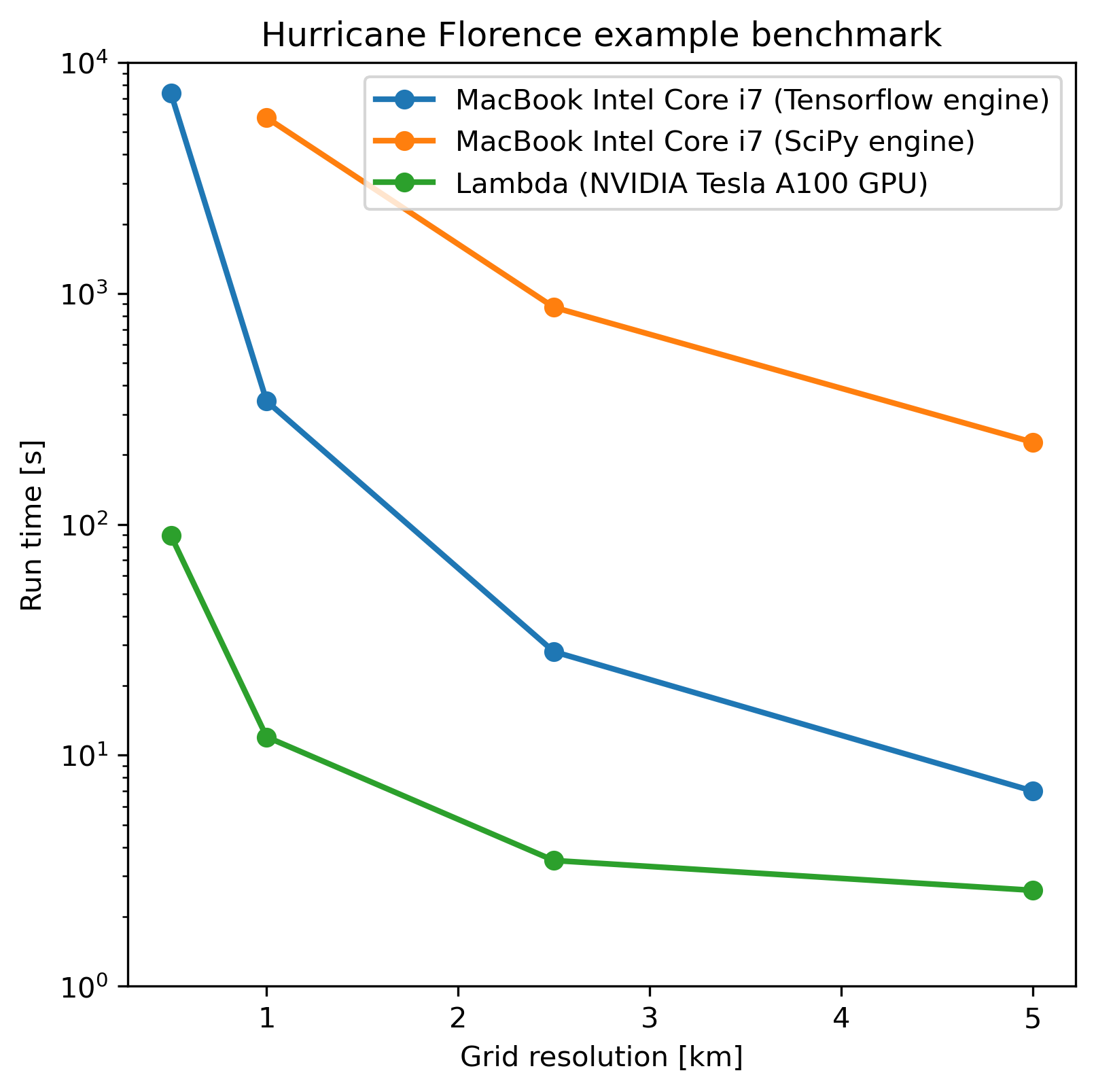
Figure 1:The time in seconds of execution of the Hurricane Florence retrieval example when using the TensorFlow and SciPy engines on an Intel Core i7 MacBook in CPU mode and on a node of Argonne National Laboratory’s Lambda cluster, utilizing a single NVIDIA Tesla A100 GPU for the calculation.
| Method | 0.5 km | 1 km | 2.5 km | 5.0 km |
|---|---|---|---|---|
| SciPy Engine | ~50 days | 5771.2 s | 871.5 s | 226.9 s |
| TensorFlow Engine | 7372.5 s | 341.5 s | 28.1 s | 7.0 s |
| NVIDIA Tesla A100 GPU | 89.4 s | 12.0 s | 3.5 s | 2.6 s |
Figure 1 and Table 1 show that, in general, the retrievals took anywhere from 10 to 100 fold less time on the GPU compared to the CPU. The discrepancy in performance between the GPU and CPU-based retrievals increases as resolution decreases, demonstrating the importance of the GPU for conducting high-resolution wind retrievals. In Table 1, using a GPU to retrieve the Hurricane Florence example at 1 km resolution reduces the run time from 341 s to 12 s. Therefore, these performance improvements show that PyDDA’s TensorFlow-based engine now enables it to handle both spatial scales of hundreds of kms at a 1 km resolution. For a day of data at this resolution, assuming five minutes between scans, an entire day of data can be processed in 57 minutes. With the use of multi-GPU clusters and selecting for cases where precipitation is present, this enables the ability to process winds from multi-year radar datasets within days instead of months.
In addition, simply using TensorFlow’s implementation of L-BFGS-B as well as the TensorFlow calculated cost function and gradients provides a significant performance improvement compared to the original “scipy” engine in PyDDA 0.5, being up to a factor of 30 faster. In fact, running PyDDA’s original “scipy” engine on the 0.5 km resolution data for the Hurricane Florence example would have likely taken 50 days to complete on an Intel Core i7-based MacBook laptop. Therefore, that particular run was not tenable to do and therefore not shown in Figure 1. In any case, this shows that upgrading the calculations to use TensorFlow’s automatically generated gradients and L-BFGS-B implementation provides a very significant speedup to the processing time.
Augmented Lagrangian method
The release of PyDDA 1.0 focused on improving its performance and gradient accuracy by using automatic differentiation for calculating the gradient. For PyDDA 1.1, the PyDDA development team focused on implementing a technique that enables the user to automatically determine the weight coefficients μ. This technique builds upon the automatic differentiation work done for PyDDA 1.0 by using the automatically generated gradients. In this work, we consider a constrained reformulation of (4) that requires wind fields returned by PyDDA to (approximately) satisfy mass continuity constraints. That is, we focus on the constrained optimization problem
where we now interpret as a vector mapping that outputs, at each grid point in the discretized volume . Notice that the formulation in (5) has no dependencies on scalars μ.
To solve the optimization problem in (5), we implemented an augmented Lagrangian method with a filter mechanism inspired by Leyffer & Vanaret (2020). An augmented Lagrangian method considers the Lagrangian associated with an equality-constrained optimization problem, in this case , where λ is a vector of Lagrange multipliers of the same length as the number of grid points in the discretized volume. The Lagrangian is then augmented with an additional squared-penalty term on the constraints to yield , where we have intentionally used as the scalar in the penalty term to make comparisons with (4) transparent. It is well known (see, for instance, Theorem 17.5 of Nocedal & Wright (2006)) that under some not overly restrictive conditions there exists a finite such that if , then each local solution of (5) corresponds to a strict local minimizer of for a suitable choice of multipliers . Essentially, augmented Lagrangian methods solve a short sequence of unconstrained problems , with different values of μ until a solution is returned that is a local, feasible solution to (5). In our implementation of an augmented Lagrangian method, the coarse minimization of is performed by the Scipy implementation of LBFGS-B with the TensorFlow implementation of the cost function and gradients. Additionally, in our implementation, we employ a filter mechanism (see a survey in Fletcher et al. (2006)) recently proposed for augmented Lagrangian methods in Leyffer & Vanaret (2020) in order to guarantee convergence. We defer details to that paper, but note that the feasibility restoration phase (the minimization of a squared constraint violation) required by such a filter method is also performed by the SciPy implementation of LBFGS-B.
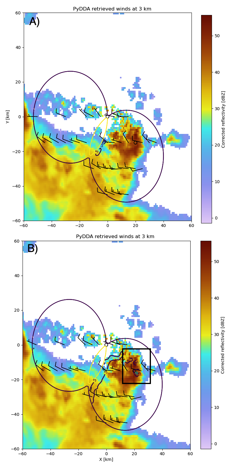
Figure 2:The PyDDA retrieved winds overlaid over reflectivity from the C-band Polarization Radar for the MCS that passed over Darwin, Australia on 20 Jan 2006. The winds were retrieved using the weak variational technique with (a) and the Augmented Lagrangian technique with (b). The contours represent vertical velocities at 3.05 km altitude. The boxed region shows the updrafts that generated the heavy precipitation.
The PyDDA documentation contains an example of a mesoscale convective system (MCS) that was sampled by a C-band Polarization Radar (CPOL) and a Bureau of Meteorology Australia radar on 20 Jan 2006 in Darwin, Australia. For more details on this storm and the radar network configuration, see Collis et al. (2013). For more information about the CPOL radar dataset, see Jackson et al. (2018). This example with its data is included in the PyDDA Documentation as the “Example of retrieving and plotting winds.”
Figure 2 shows the winds retrieved by the Augmented Lagrangian technique with and from the weak variational technique with on the right. Figure 2 shows that both techniques are capturing similar horizontal wind fields in this storm. However, the Augmented Lagrangian technique is resolving an updraft that is not present in the wind field generated by the weak variational technique. Since there is horizontal wind convergence in this region, we expect there to be an updraft present in this box in order for the solution to be physically realistic. Therefore, for , the Augmented Lagrangian technique is doing a better job at resolving the updrafts present in the storm than the weak variational technique is. This shows that adjusting μ is required in order for the weak variational technique to resolve the updraft.
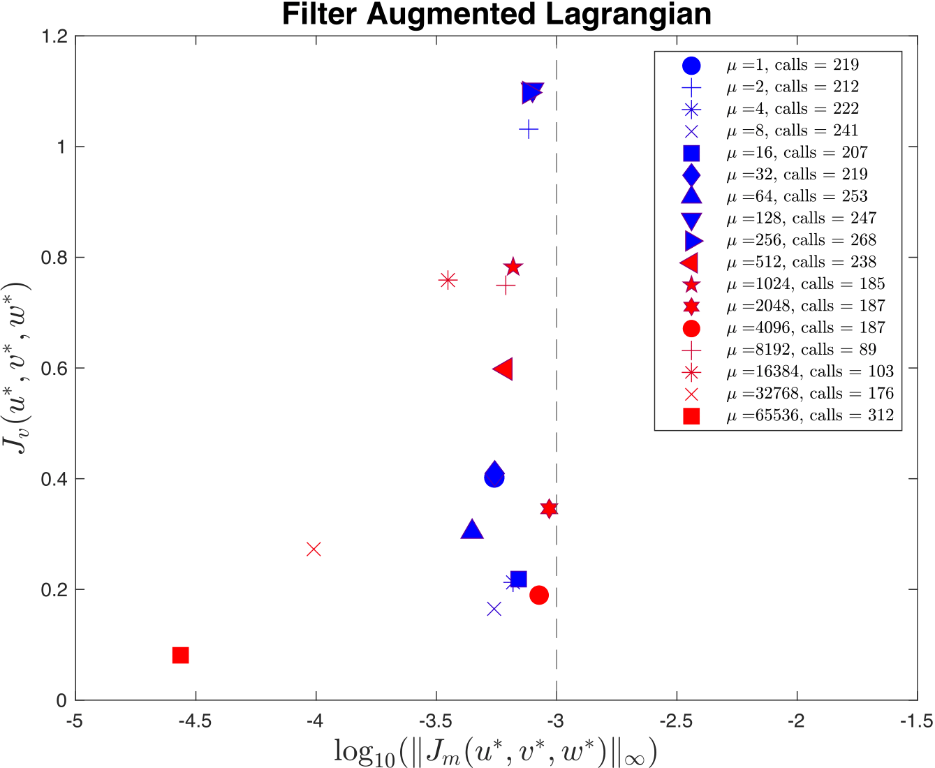
Figure 3:The -axis shows, on a logarithmic scale, the maximum constraint violation in the units of divergence of the wind field and the -axis shows the value of the data-fitting term at the optimal solution. The legend lists the number of function/gradient calls made by the filter Augmented Lagrangian Method, which is the dominant cost of both approaches. The dashed line at 10-3 denotes the tolerance on the maximum constraint violation that was supplied to the filter Augmented Lagrangian method.
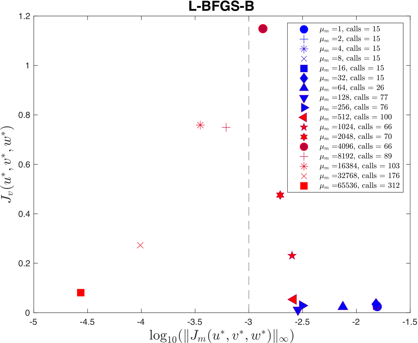
Figure 4:As Figure 3, but for the weak variational technique that uses L-BFGS-B.
We solve the unconstrained formulation (4) using the implementation of L-BFGS-B currently employed in PyDDA; we fix the value and vary . We also solve the constrained formulation (5) using our implementation of a filter Augmented Lagrangian method, and instead vary the initial guess of penalty parameter . For the initial state, we use the wind profile from the weather balloon launch at 00 UTC 20 Jan 2006 from Darwin and apply it to the whole analysis domain. A summary of results is shown in Figure 3 and Figure 4. We applied a maximum constraint violation tolerance of 10-3 to the filter Augmented Lagrangian method. This is a tolerance that assumes that the winds do not violate the mass continuity constraint by more than . Notice that such a tolerance is impossible to supply to the weak variational method, highlighting the key advantage of employing a constrained method. Notice that in this example, only 5 settings of lead to sufficiently feasible solutions returned by the variational technique.
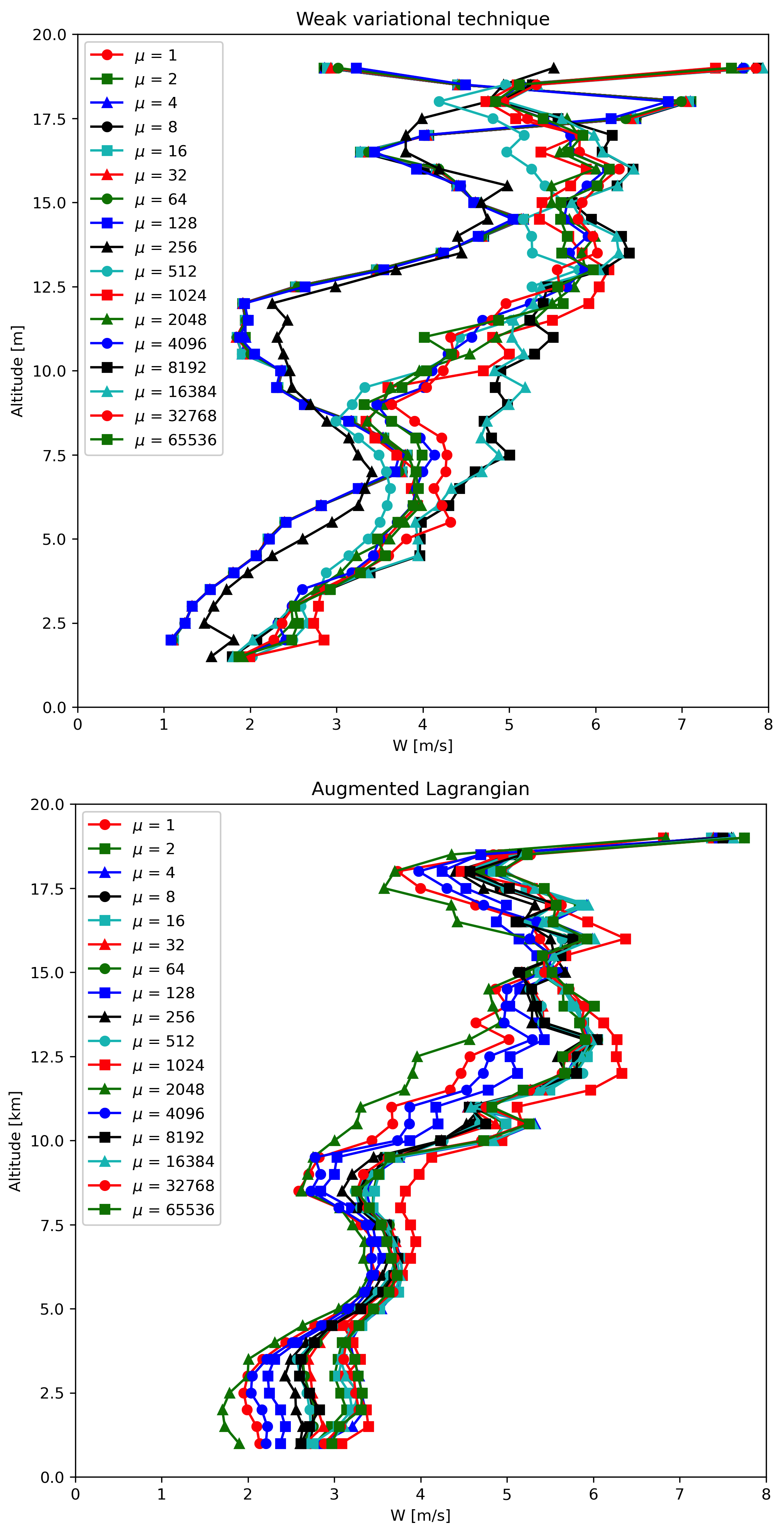
Figure 5:The mean updraft velocity obtained by (left) the weak variational and (right) the Augmented Lagrangian technique inside the updrafts in the boxed region of Figure 2. Each line represents a different value of μ for the given technique.
Table 2:Minimum, mean, maximum, and standard deviation of (m/s) for select levels in Figure 5.
| Min | Mean | Max | Std. Dev. | |
|---|---|---|---|---|
| Weak variational | ||||
| 2.5 km | 1.2 | 1.8 | 2.7 | 0.6 |
| 5 km | 2.2 | 2.9 | 4.0 | 0.7 |
| 7.5 km | 3.2 | 3.9 | 5.0 | 0.4 |
| 10 km | 2.3 | 3.3 | 4.9 | 1.0 |
| Aug. Lagrangian | ||||
| 2.5 km | 1.8 | 2.8 | 3.3 | 0.5 |
| 5 km | 3.1 | 3.3 | 3.5 | 0.1 |
| 7.5 km | 3.2 | 3.5 | 3.9 | 0.1 |
| 10 km | 3.0 | 4.3 | 4.9 | 0.5 |
Finally, a variable of interest to atmospheric scientists for winds inside MCSes is the vertical wind velocity. It provides a measure of the intensity of the storm by demonstrating the amount of upscale growth contributing to intensification. Figure 5 shows the mean updraft velocities inside the box in Figure 2 as a function of height for each of the runs of the TensorFlow L-BFGS-B and Augmented Lagrangian techniques. Table 2 summarizes the mean and spread of the solutions in Figure 5. For the updraft velocities produced by the Augmented Lagrangian technique, there is a 1 m/s spread of velocities produced for given values of μ at altitudes < 7.5 km in Table 2. At an altitude of 10 km, this spread is 1.9 m/s. This is likely due to the reduced spatial coverage of the radars at higher altitudes. However, for the weak variational technique, the sensitivity of the retrieval to μ is much more pronounced, with up to 2.8 m/s differences between retrievals. Therefore, using the Augmented Lagrangian technique makes the vertical velocities less sensitive to μ. Therefore, this shows that using the Augmented Lagrangian technique will result in more reproducible wind fields from radar wind networks since it is less sensitive to user-defined parameters than the weak variational technique. However, a limitation of this technique is that, for now, this technique is limited to two radars and to the mass continuity and vertical vorticity constraints.
Concluding remarks
Atmospheric wind retrievals are vital for forecasting severe weather events. Therefore, this motivated us to develop an open source package for developing atmospheric wind retrievals called PyDDA. In the original releases of PyDDA (versions 0.5 and prior), the original goal of PyDDA was to convert legacy wind retrieval packages such as CEDRIC and Multidop to be fully Pythonic, open source, and accessible to the scientific community. However, there remained many improvements to be made to PyDDA to optimize the speed of the retrievals and to make it easier to add constraints to PyDDA.
This therefore motivated two major changes to PyDDA’s wind retrieval routine for PyDDA 1.0. The first major change to PyDDA in PyDDA 1.0 was to simplify the wind retrieval process by automating the calculation of the gradient of the cost function used for the weak variational technique. To do this, we utilized Jax and TensorFlow’s capabilities to do automatic differentiation of functions. This also allows PyDDA to take advantage of GPU resources, significantly speeding up retrieval times for mesoscale retrievals at kilometer-scale resolution. In addition, running the TensorFlow-based version of PyDDA provided significant performance improvements even when using a CPU.
These automatically generated gradients were then used to implement an Augmented Lagrangian technique in PyDDA 1.1 that allows for automatically determining the weights for each cost function in the retrieval. The Augmented Lagrangian technique guarantees convergence to a physically realistic solution, something that is not always the case for a given set of weights for the weak variational technique. Therefore, this both creates more reproducible wind retrievals and simplifies the process of retrieving winds for the non-specialist user. However, since the Augmented Lagrangian technique currently only supports the ingesting of radar data into the retrieval, plans for PyDDA 1.2 and beyond include expanding the Augmented Lagrangian technique to support multiple data sources such as models and rawinsondes.
Code Availability
PyDDA is available for public use with documentation and examples available at https://
The submitted manuscript has been created by UChicago Argonne, LLC, Operator of Argonne National Laboratory (‘Argonne’). Argonne, a U.S. Department of Energy Office of Science laboratory, is operated under Contract No. DE-AC02-06CH11357. The U.S. Government retains for itself, and others acting on its behalf, a paid-up nonexclusive, irrevocable worldwide license in said article to reproduce, prepare derivative works, distribute copies to the public, and perform publicly and display publicly, by or on behalf of the Government. The Department of Energy will provide public access to these results of federally sponsored research in accordance with the DOE Public Access Plan. This material is based upon work supported by Laboratory Directed Research and Development (LDRD) funding from Argonne National Laboratory, provided by the Director, Office of Science, of the U.S. Department of Energy under Contract No. DE-AC02-06CH11357. This material is also based upon work funded by program development funds from the Mathematics and Computer Science and Environmental Science departments at Argonne National Laboratory.
Copyright © 2022 Jackson et al. This is an open-access article distributed under the terms of the Creative Commons Attribution 3.0 Unported license.
- CPOL
- C-band Polarization Radar
- MCS
- mesoscale convective system
- Shapiro, A., Potvin, C. K., & Gao, J. (2009). Use of a Vertical Vorticity Equation in Variational Dual-Doppler Wind Analysis. Journal of Atmospheric and Oceanic Technology, 26(10), 2089–2106. 10.1175/2009JTECHA1256.1
- Potvin, C. K., Shapiro, A., & Xue, M. (2012). Impact of a Vertical Vorticity Constraint in Variational Dual-Doppler Wind Analysis: Tests with Real and Simulated Supercell Data. Journal of Atmospheric and Oceanic Technology, 29(1), 32–49. 10.1175/JTECH-D-11-00019.1
- Miller, L. Jay, & Fredrick, S. M. (1998). Custom Editing and Display of Reduced Information in Cartesian space [Techreport]. National Center for Atmospheric Research.
- Lang, T., Souto, M., Khobahi, S., & Jackson, B. (2017). nasa/MultiDop: MultiDop v0.3 (v0.3) [Computer software]. Zenodo. 10.5281/zenodo.1035904
- Jackson, R., Collis, S., Lang, T., Potvin, C., & Munson, T. (2020). PyDDA: A Pythonic Direct Data Assimilation Framework for Wind Retrievals. Journal of Open Research Software, 8(1), 20. 10.5334/jors.264
- Robert Jackson, Scott Collis, Timothy Lang, Corey Potvin, & Todd Munson. (2019). PyDDA: A new Pythonic Wind Retrieval Package. In Chris Calloway, David Lippa, Dillon Niederhut, & David Shupe (Eds.), Proceedings of the 18th Python in Science Conference (pp. 111–117). 10.25080/Majora-7ddc1dd1-010
- Harris, C. R., Millman, K. J., van der Walt, S. J., Gommers, R., Virtanen, P., Cournapeau, D., Wieser, E., Taylor, J., Berg, S., Smith, N. J., Kern, R., Picus, M., Hoyer, S., van Kerkwijk, M. H., Brett, M., Haldane, A., del Río, J. F., Wiebe, M., Peterson, P., … Oliphant, T. E. (2020). Array programming with NumPy. Nature, 585(7825), 357–362. 10.1038/s41586-020-2649-2
- Virtanen, P., Gommers, R., Oliphant, T. E., Haberland, M., Reddy, T., Cournapeau, D., Burovski, E., Peterson, P., Weckesser, W., Bright, J., van der Walt, S. J., Brett, M., Wilson, J., Millman, K. J., Mayorov, N., Nelson, A. R. J., Jones, E., Kern, R., Larson, E., … SciPy 1.0 Contributors. (2020). SciPy 1.0: Fundamental Algorithms for Scientific Computing in Python. Nature Methods, 17, 261–272. 10.1038/s41592-019-0686-2
- Bradbury, J., Frostig, R., Hawkins, P., Johnson, M. J., Leary, C., Maclaurin, D., Necula, G., Paszke, A., VanderPlas, J., Wanderman-Milne, S., & Zhang, Q. (2018). JAX: composable transformations of Python+NumPy programs (0.2.5) [Computer software]. http://github.com/google/jax
- Abadi, M., Agarwal, A., Barham, P., Brevdo, E., Chen, Z., Citro, C., Corrado, G. S., Davis, A., Dean, J., Devin, M., Ghemawat, S., Goodfellow, I., Harp, A., Irving, G., Isard, M., Jia, Y., Jozefowicz, R., Kaiser, L., Kudlur, M., … Zheng, X. (2015). TensorFlow: Large-Scale Machine Learning on Heterogeneous Systems. https://www.tensorflow.org/
- Liu, D. C., & Nocedal, J. (1989). On the limited memory BFGS method for large scale optimization. MATHEMATICAL PROGRAMMING, 45, 503–528. 10.1007/bf01589116
- Leyffer, S., & Vanaret, C. (2020). An augmented Lagrangian filter method. Mathematical Methods of Operations Research, 92(2), 343–376. 10.1007/s00186-020-00713-x
- Nocedal, J., & Wright, S. J. (2006). Numerical Optimization (second). Springer.
- Fletcher, R., Leyffer, S., & Toint, P. (2006). A brief history of filter methods [Techreport]. Argonne National Laboratory. http://www.optimization-online.org/DB_FILE/2006/10/1489.pdf
- Collis, S., Protat, A., May, P. T., & Williams, C. (2013). Statistics of Storm Updraft Velocities from TWP-ICE Including Verification with Profiling Measurements. Journal of Applied Meteorology and Climatology, 52(8), 1909–1922. 10.1175/JAMC-D-12-0230.1
