
Variational Autoencoders For Semi-Supervised Deep Metric Learning
Abstract
Deep metric learning (DML) methods generally do not incorporate unlabelled data. We propose borrowing components of the variational autoencoder (VAE) methodology to extend DML methods to train on semi-supervised datasets. We experimentally evaluate the atomic benefits to the perform- ing DML on the VAE latent space such as the enhanced ability to train using unlabelled data and to induce bias given prior knowledge. We find that jointly training DML with an autoencoder and VAE may be potentially helpful for some semi-supervised datasets, but that a training routine of alternating between the DML loss and an additional unsupervised loss across epochs is generally unviable.
Introduction
Within the broader field of representation learning, metric learning is an area which looks to define a distance metric which is smaller between similar objects (such as objects of the same class) and larger between dissimilar objects. Oftentimes, a map is learned from inputs into a low-dimensional latent space where euclidean distance exhibits this relationship, encouraged by training said map against a loss (cost) function based on the euclidean distance between sets of similar and dissimilar objects in the latent space. Existing metric learning methods are generally unable to learn from unlabelled data, which is problematic because unlabelled data is often easier to obtain and is potentially informative.
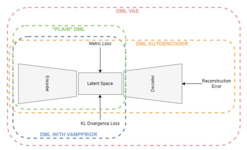
We take inspiration from variational autoencoders (VAEs), a generative representation learning architecture, for using unlabelled data to create accurate representations. Specifically, we look to evaluate three atomic improvement proposals that detail how pieces of the VAE architecture can create a better deep metric learning (DML) model on a semi-supervised dataset. From here, we can ascertain which specific qualities of how VAEs process unlabelled data are most helpful in modifying DML methods to train with semi-supervised datasets.
First, we propose that the autoencoder structure of the VAE helps the clustering of unlabelled points, as the reconstruction loss may help incorporate semantic information from unlabelled sources. Second, we propose that the structure of the VAE latent space, as it is confined by a prior distribution, can be used to induce bias in the latent space of a DML system. For instance, if we know a dataset contains N-many classes, creating a prior distribution that is a learnable mixture of N gaussians may help produce better representations. Third, we propose that performing DML on the latent space of the VAE so that the DML task can be jointly optimized with the VAE to incorporate unlabelled data may help produce better representations.
Each of the three improvement proposals will be evaluated experimentally. The improvement proposals will be evaluated by comparing a standard DML implementation to the same DML implementation:
- jointly optimized with an autoencoder
- while structuring the latent space around a prior distribution using the VAE’s KL-divergence loss term between the approximated posterior and prior
- jointly optimized with a VAE
Our primary contribution is evaluating these three improvement proposals. Our secondary contribution is presenting the results of the joint approaches for VAEs and DML for more recent metric losses that have not been jointly optimized with a VAE in previous literature.
Related Literature
The goal of this research is to investigate how components of the variational autoencoder can help the performance of deep metric learning in semi supervised tasks. We draw on previous literature to find not only prior attempts at this specific research goal but also work in adjacent research questions that proves insightful. In this review of the literature, we discuss previous related work in the areas of Semi-Supervised Metric Learning and VAEs with Metric Losses.
Semi-Supervised Metric Learning
There have been previous approaches to designing metric learning architectures which incorporate unlabelled data into the metric learning training regimen for semi-supervised datasets. One of the original approaches is the MPCK-MEANS algorithm proposed by Bilenko et al. (2004), which adds a penalty for placing labelled inputs in the same cluster which are of a different class or in different clusters if they are of the same class. This penalty is proportional to the metric distance between the pair of inputs. Baghshah & Shouraki (2009) also looks to impose similar constraints by introducing a loss term to preserve locally linear relationships between labelled and unlabelled data in the input space. Wang et al. (2013) also use a regularizer term to preserve the topology of the input space. Using VAEs, in a sense, draws on this theme: though there is not explicit term to enforce that the topology of the input space is preserved, a topology of the inputs is intended to be learned through a low-dimensional manifold in the latent space.
One more recent common general approach to this problem is to use the unlabelled data’s proximity to the labelled data to estimate labels for unlabelled data, effectively transforming unlabelled data into labelled data. Dutta et al. (2021) and Li et al. (2019) propose a model which uses affinity propagation on a k-Nearest-Neighbors graph to label partitions of unlabelled data based on their closest neighbors in the latent space. Wu et al. (2020) also look to assign pseudo-labels to unlabelled data, but not through a graph-based approach. Instead, the proposed model looks to approximate “soft” pseudo-labels for unlabelled data from the metric learning similarity measure between the embedding of unlabelled data and the center of each input of each class of the labelled data.
Several of the recent graph based approaches can be considered state-of-the-art for semi supervised metric learning. Li et. al.'s paper states their methods achieve 98.9 percent clustering accuracy on the MNIST dataset with 10% labelled data, outperforming two similar state-of-the-art methods, DFCM Arshad et al., 2018 and SDEC Ren et al., 2019, by roughly 8 points. Dutta et. al.'s method also outperforms 5 other state for the R@1 metric (the “percentage of test examples” that have at least one 1 “nearest neighbor from the same class.”) by at least 1.2 on the MNIST dataset, as well as the Fashion-MNIST and CIFAR-10 datasets. It is difficult to compare the two approaches as the evaluation metrics used in each paper differ. Li et al.'s paper has been cited rather heavily relative to other papers in the field and can be considered state of the art for semi-supervised DML on MNIST. The paper also provides a helpful metric (98.9 percent clustering accuracy on the MNIST dataset with 10% labelled data) to use as a reference point for the results in this paper.
VAEs with Metric Loss
Some approaches to incorporating labelled data into VAEs use a metric loss to govern the latent space more explicitly. Lin et al. (2018) model the intra-class invariance (i.e. the class-related information of a data point) and intra-class variance (i.e. the distinct features of a data point not unique to it’s class) seperately. Like several other models in this section, this paper’s proposed model incorporates a metric loss term for the latent vectors representing intra-class invariance and the latent vectors representing both intra-class invariance and intra-class variance.
Kulkarni et al. (2020) incorporate labelled information into the VAE methodology in two ways. First, a modified architecture called the CVAE is used in which the encoder and generator of the VAE is not only conditioned on the input and latent vector , respectively, but also on the label . The CVAE was introduced in previous papers Sohn et al., 2015Dahmani et al., 2019. Second, the authors add a metric loss, specifically a multi-class N-pair loss Sohn, 2016, in the overall loss function of the model. While it is unclear how the CVAE technique would be adapted in a semi-supervised setting, as there is not a label associated with each datapoint , we also experiment with adding a (different) metric loss to the overall VAE loss function.
Most recently, Grosnit et al. (2021) leverage a new training algorithm for combining VAEs and DML for Bayesian Optimization and said algorithm using simple, contrastive, and triplet metric losses. We look to build on this literature by also testing a combined VAE DML architecture on more recent metric losses, albeit using a simpler training regimen.
Deep Metric Learning (DML)
Metric learning attempts to create representations for data by training against the similarity or dissimilarity of samples. In a more technical sense, there are two notable functions in DML systems. Function is a neural network which maps the input data to the latent points (i.e. , where θ is the network parameters). Generally, exists in a space of much lower dimensionality than (eg. is a set of pixel pictures such that and ).
The function represents the distance between two inputs . To create a useful embedding model , we would like for to produce large values of when and are dissimilar and for to produce small values of when and are similar. In some cases, dissimilarity and similarity can refer to when inputs are of different and the same classes, respectively.
It is common for the Euclidean metric (i.e. the metric) to be used as a distance function in metric learning. The generalized metric can be defined as follows, where .
If we have chosen (a neural network) and the distance function (the metric), the remaining component to be defined in a metric learning system is the loss function for training . In practice, we will be using triplet loss Schroff et al., 2015, one of the most common metric learning loss functions.
Methodology
We look to discover the potential of applying components of the VAE methodology to DML systems. We test this through presenting incremental modifications to the basic DML architecture. Each modified architecture corresponds to an improvement proposal about how a specific part of the VAE training regime and loss function may be adapted to assist the performance of a DML method for a semi-supervised dataset.

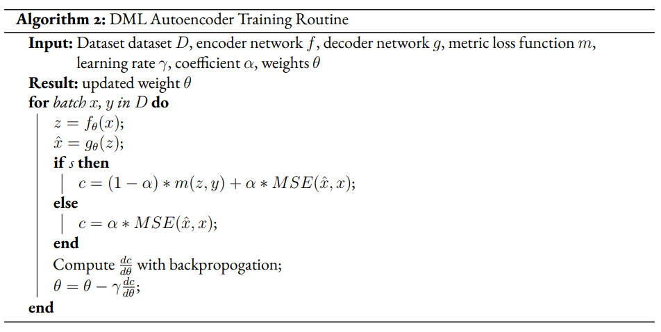
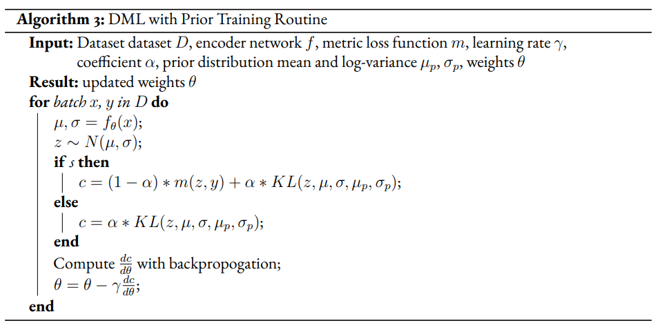
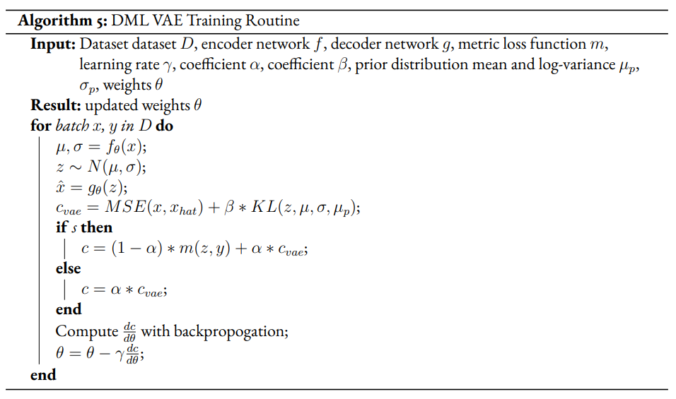
The general method we will take for creating modified DML models involves extending the training regimen to two phases, a supervised and unsupervised phase. In the supervised phase the modified DML model behaves identically to the base DML model, training on the same metric loss function. In the unsupervised phase, the DML model will train against an unsupervised loss inspired by the VAE. This may require extra steps to be added to the DML architecture. In the pseudocode, refers to boolean variable representing if the current phase is supervised. α is a hyperparameter which modulates the impact of the unsupervised on total loss for the DML autoencoder.
Improvement Proposal 1
We first look to evaluate the improvement proposal that adding a reconstruction loss to a DML system can improve the quality of clustering in the latent representations on a semi-supervised dataset. Reconstruction loss in and of itself enforces a similar semantic mapping onto the latent space as a metric loss, but can be computed without labelled data. In theory, we believe that the added constraint that the latent vector must be reconstructed to approximate the original output will train the spatial positioning to reflect semantic information. Following this reasoning, observations which share similar semantic information, specifically observations of the same class (even if not labelled as such), should intuitively be positioned nearby within the latent space. To test if this intuition occurs in practice, we evaluate if a DML model with an autoencoder structure and reconstruction loss (described in further detail below) will perform better than a plain DML model in terms of clustering quality. This will be especially evident for semi-supervised datasets in which the amount of labelled data is not feasible for solely supervised DML.
Given a semi-supervised dataset, we assume a standard DML system will use only the labelled data and train given a metric loss (see Algorithm 1). Our modified model DML Autoencoder will extend the DML model’s training regime by adding a decoder network which takes the latent point as input and produces an output . The unsupervised loss is equal to the reconstruction loss.
Improvement Proposal 2
Say we are aware that a dataset has classes. It may be useful to encourage that there are clusters in the latent space of a DML model. This can be enforced by using a prior distribution containing many Gaussians. As we wish to measure only the affect of inducing bias on the representation without adding any complexity to the model, the prior distribution will not be learnable (unlike VAE with VampPrior). By testing whether the classes of points in the latent space are organized along the prior components we can test whether bias can be induced using a prior to constrain the latent space of a DML. By testing whether clustering improves performance, we can evaluate whether this inductive bias is helpful.
Given a fully supervised dataset, we assume a standard DML system will use only the labelled data and train given a metric loss . Our modified model will extend the DML system’s training regime by setting the unsupervised loss to a KL divergence term that measures the difference between posterior distributions and a prior distribution. It should also be noted that, like the VAE encoder, we will map the input not to a latent point but to a latent distribution. The latent point is stochastically sampled from the latent distribution during training. Mapping the input to a distribution instead of a point will allow us to calculate the KL divergence.
In practice, we will be evaluating a DML model with a unit prior and a DML model with a mixture of gaussians (GMM) prior. The latter model constructs the prior as a mixture of gaussians – each the vertex of the unit (i.e. each side is 2 units long) hypercube in the latent space. The logvar of each component is set equal to one. Constructing the prior in this way is beneficial in that it is ensured that each component is evenly spaced within the latent space, but is limiting in that there must be exactly components in the GMM prior. Thus, to test, we will test a dataset with 10 classes on the latent space dimensionality of 4, such that there are gaussian components in the GMM prior. Though the number of prior components is greater than the number of classes, the latent mapping may still exhibit the pattern of classes forming clusters around the prior components as the extra components may be made redundant.
The drawback of the decision to set the GMM components’ means to the coordinates of the unit hypercube’s vertices is that the manifold of the chosen dataset may not necessarily exist in 4 dimensions. Choosing gaussian components from a d-dimensional hypersphere in the latent space would solve this issue, but there does not appear to be a solution for choosing evenly spaced points spanning dimensions on a -dimensional hypersphere. KL Divergence is calculated with a monte carlo approximation for the GMM and analytically with the unit prior.

Improvement Proposal 3
The third improvement proposal we look to evaluate is that given a semi-supervised dataset, optimizing a DML model jointly with a VAE on the VAE’s latent space will produce superior clustering than the DML model individually. The intuition behind this approach is that DML methods can learn from only supervised data and VAE methods can learn from only unsupervised data; the proposed methodology will optimize both tasks simultaneously to learn from both supervised and unsupervised data.
The MetricVAE implementation we create jointly optimizes the VAE task and DML task on the VAE latent space. The unsupervised loss is set to the VAE loss. The implementation uses the VAE with VampPrior model instead of the vanilla VAE.
Results
Experimental Configuration
Each set of experiments shares a similar hyperparameter search space. Below we describe the hyperparameters that are included in the search space of each experiment and the evaluation method.
Learning Rate (lr)
Through informal experimentation, we have found that the learning rate of 0.001 causes the models to converge consistently (relative to 0.005 and 0.0005). The learning rate is thus set to 0.001 in each experiment.
Latent Space Dimensionality (lsdim)
Latent space dimensionality refers to the dimensionality of the vector output of the encoder of a DML network or the dimensionality of the posterior distribution of a VAE (also the dimensionality of the latent space). When the latent space dimensionality is 2, we see the added benefit of creating plots of the latent representations (though we can accomplish this through using dimensionality reduction methods like tSNE for higher dimensionalities as well). Example values for this hyperparameter used in experiments are 2, 4, and 10.
Alpha
Alpha (α) is a hyperapameter which refers to the balance between the unsupervised and supervised losses of some of the modified DML models. More details about the role of α in the model implementations are discussed in the methodology section of the model. Potential values for alpha are each between 0 (exclusive) and 1 (inclusive). We do not include 0 in this set as if α is set to 0, the model is equivalent to the fully supervised plain DML model because the supervised loss would not be included. If α is set to 1, then the model would train on only the unsupervised loss; for instance if the DML Autoencoder had α set to 1, then the model would be equivalent to an autoencoder.
Partial Labels Percentage (pl%)
The partial labels percentage hyperparameter refers to the percentage of the dataset that is labelled and thus the size of the portion of the dataset that can be used for labelled training. Of course, each of the datasets we use is fully labelled, so a partially labelled dataset can be trivially constructed by ignoring some of the labels. As the sizes of the dataset vary, each percentage can refer to a different number of labelled samples. Values for the partial label percentage we use across experiments include 0.01, 0.1, and 10 (with each value referring to the percentage).
Datasets
Two datasets are used for evaluating the models. The first dataset is MNIST LeCun & Cortes, 2010, a very popular dataset in machine learning containing greyscale images of handwritten digits. The second dataset we use is the organ OrganAMNIST dataset from MedMNIST v2 Yang et al., 2021. This dataset contains 2D slices from computed tomography images from the Liver Tumor Segmentation Benchmark – the labels correspond to the classification of 11 different body organs. The decision to use a second dataset was motivated because as the improvement proposals are tested over more datasets, the results supporting the improvement proposals become more generalizable. The decision to use the OrganAMNIST dataset specifically is motivated in part due to the Quinn Research Group working on similar tasks for biomedical imaging Zain et al., 2020. It is also motivated in part because OrganAMNIST is a more difficult dataset, at least for the classfication task, as the leading accuracy for MNIST is .9991 An et al., 2020 while the leading accuracy for OrganAMNIST is .951 Yang et al., 2021. The MNIST and OrganAMNIST datasets are similar in dimensionality (1 x 28 x 28), number of samples (60,000 and 58,850, respectively) and in that they are both greyscale.
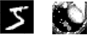
Figure 1:Sample images from the MNIST (left) and OrganAMNIST of MedMNIST (right) datasets
Evaluation
We evaluate the results by running each model on a test partition of data. We then take the latent points generated by the model and the corresponding labels . Three classifiers (sklearn’s implementation of RandomForest, MLP, and kNN) each output predicted labels for the latent points. In most of the charts shown, however, we only include the kNN classification output due to space constraints and the lack of meaningful difference between the output for each classifier. We finally measure the quality of the predicted labels using the Adjusted Mutual Information Score (AMI) Vinh et al., 2010 and accuracy (which is still helpful but is also easier to interpret in some cases). This scoring metric is common in research that looks to evaluate clustering performance Zhu & Gao, 2021Emmons et al., 2016. We will be using sklearn’s implementation of AMI Pedregosa et al., 2011. The performance of a classifier on the latent points intuitively can be used as a measure of quality of clustering.
Improvement Proposal 1 Results: Benefits of Reconstruction Loss
In evaluating the first improvement proposal, we compare the performance of the plain DML model to the DML Autoencoder model. We do so by comparing the performance of the plain DML system and the DML Autoencoder across a search space containing the lsdim, alpha, and pl% hyperparameters and both datasets.
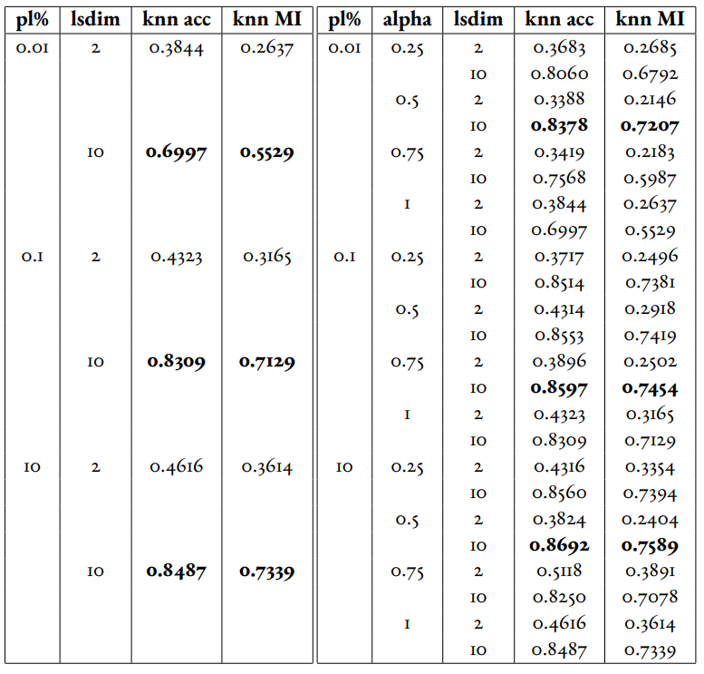
In Table 1 and Table 2, we observe that for relatively small amounts of labelled samples (the partial labels percentages of 0.01 and 0.1 correspond to 6 and 60 labelled samples respectively), the DML Autoencoder severely outperforms the DML model. However, when the number of labelled samples increases (the partial labels percentage of 10 correspond to 6000 labelled samples respectively), the DML model significantly outperforms the DML Autoencoder. This trend is not too surprising, as when there is sufficient data to train unsupervised methods and insufficient data to train supervised method, as is the case for the 0.01 and 0.1 partial label percentages, the unsupervised method will likely perform better.
The data looks to show that adding a reconstruction loss to a DML system can improve the quality of clustering in the latent representations on a semi-supervised dataset when there are small amounts (roughly less than 100 samples) of labelled data and a sufficient quantity of unlabelled data. But an important caveat is that it is not convincing that the DML Autoencoder effectively combined the unsupervised and supervised losses to create a superior model, as a plain autoencoder (i.e. the DML Autoencoder with ) outperforms the DML for the partial labels percentage of or less than 0.1% and underperforms the DML for the partial labels percentage of 10%.
Table 1:Comparison of the DML (left) and DML Autoencoder (right) models for the MNIST dataset. Bolded values indicate best performance for each partial labels percentage partition (pl%).
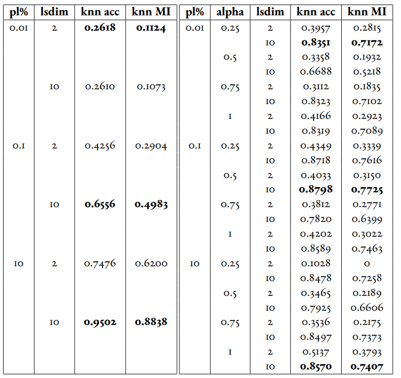
Table 2:Comparison of the DML (left) and DML Autoencoder (right) models for the MEDMNIST dataset.
Improvement Proposal 2 Results: Incorporating Inductive Bias with a Prior
In evaluating the second improvement proposal, we compare the performance of the plain DML model to the DML with a unit prior and a DML with a GMM prior. The DML prior with the GMM prior will have 2^2 = 4 gaussian components when lsdim = 2 and 2^4 = 16 components when lsdim = 4. Our broad intention is to see if changing the shape (specifically the number of components) of the prior can induce bias by affecting the pattern of embeddings. We hypothesize that when the GMM prior contains n components and n is slightly greater than or equal to the number of classes, each class will cluster around one of the prior components. We will test this for the GMM prior with 16 components (lsdim = 4) as both the MNIST and MedMNIST datasets have 10 classes. We are unable to set the number of GMM components to 10 as our GMM sampling method only allows for the number of components to equal a power of 2. Bseline models include a plain DML and a DML with a unit prior (the distribution N(0, 1)).
In Table 3, it is very evident that across both datasets, the DML models with any prior distribution all devolve to the null model (i.e. the classifier is no better than random selection). From the visualizations of the latent embeddings, we see that the embedded data for the DML models with priors appears completely random. In the case of the GMM prior, it also does not appear to take on the shape of the prior or reflect the number of components in the prior. This may be due to the training routine of the DML models. As the KL divergence loss, which can be said to “fit” the embeddings to the prior, trains on alternating epochs with the supervised DML loss, it is possible that the two losses are not balanced correctly during the training process. From the discussed results, it is fair to state that adding a prior distribution to a DML model through training the model on the KL divergence between the prior and approximated posterior distributions on alternating epochs does is not an effective way to induce bias in the latent space.
Table 3:Comparison of the DML model (left) and the DML with prior models with a unit gaussian prior (center) and GMM prior (right) models for the MNIST dataset.
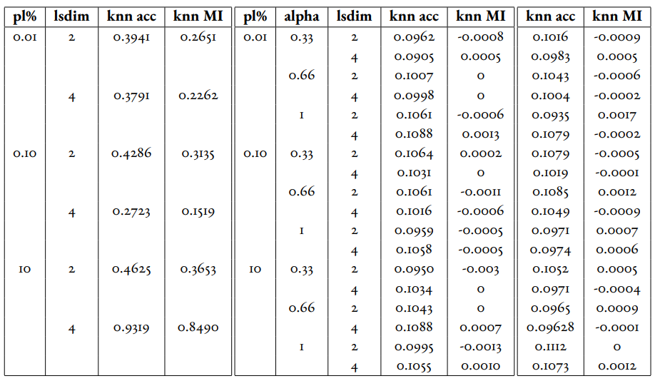
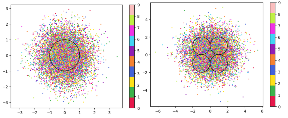
Figure 2:Comparison of latent spaces for DML with unit prior (left) and DML with GMM prior containing 4 components (right) for lsdim = 2 on OrganAMNIST dataset. The gaussian components are shown as black with the radius equal to variance (1). There appears to be no evidence of the distinct gaussian components in the latent space on the right. It does appear that the unit prior may regularize the magnitude of the latent vectors
Improvement Proposal 3 Results: Jointly Optimizing DML with VAE
To evaluate the third improvement proposal, we compare the performance of DMLs to MetricVAEs (defined in the previous chapter) across several metric losses. We run experiments for triplet loss, supervised loss, and center loss DML and MetricVAE models. To evaluate the improvement proposal, we will assess whether the model performance improves for the MetricVAE over the DML for the same metric loss and other hyper parameters.
Like the previous improvement proposal, the proposed MetricVAE model does not perform better than the null model. As with improvement proposal 2, it is possible this is because the training routine of alternating between supervised loss (in this case, metric loss) and unsupervised (in this case, VAE loss) is not optimal for training the model.
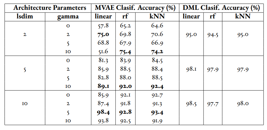
We have trained a separate combined VAE and DML model which trains on both the unsupervised and supervised loss each epoch instead of alternating between the two each epoch. In the results for this model, we see that an alpha value of over zero (i.e. incorporating both the supervised metric loss into the overall MVAE loss function) can help improve performance especially among lower dimensionalities. Given our analysis of the data, we see that incorporating the DML loss to the VAE is potentially helpful, but only when training the unsupervised and supervised losses jointly. Even in that case, it is unclear whether the MVAE performs better than the corresponding DML model even if it does perform better than the corresponding VAE model.
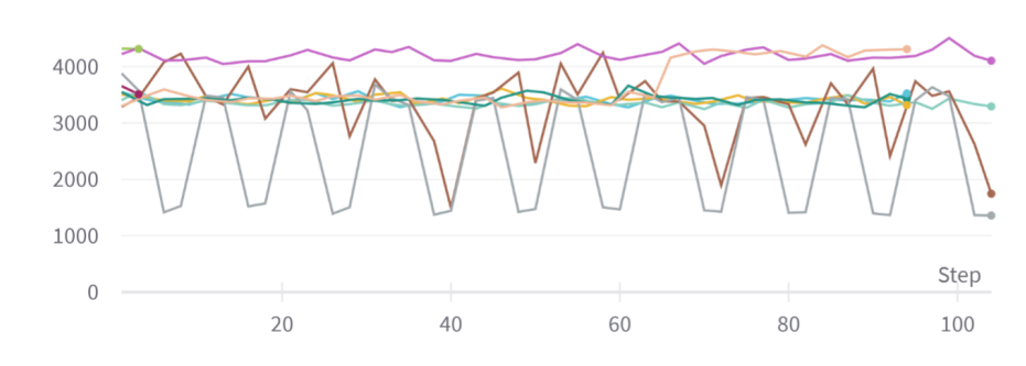
Figure 3:Graph of reconstruction loss (component of unsupervised loss) of MVAE across epochs. The unsupervised loss does not converge despite being trained on each epoch.
Table 4:Experiments performed on MVAE architecture across fully labelled MNIST dataset that trains on objective function on fully supervised dataset. The best results for the classification accuracy on the MVAE embeddings in a given latent-dimensionality are bolded.
Conclusion
Conclusion
In this work, we have set out to determine how DML can be extended for semi-supervised datasets by borrowing components of the variational autoencoder. We have formalized this approach through defining three specific improvement proposals. To evaluate each improvement proposal, we have created several variations of the DML model, such as the DML Autoencoder, DML with Unit/GMM Prior, and MVAE. We then tested the performance of the models across several semi-supervised partitions of two datasets, along with other configurations of hyperparameters.
We have determined from the analysis of our results, there is too much dissenting data to clearly accept any three of the improvement proposals. For improvement proposal 1, while the DML Autoencoder outperforms the DML for semisupervised datasets with small amounts of labelled data, it’s performance is not consistently much better than that of a plain autoencoder which uses no labelled data. For improvement proposal 2, each of the DML models with an added prior performed extremely poorly, near or at the level of the null model. For improvement proposal 3, we see the same extremely poor performance from the MVAE models.
From the results in improvement proposal 1 and 3, we find that there may be potential in incorporating the autoencoder and VAE loss terms into DML systems. However, we were unable to show that any of these improvement proposals would consistently outperform the both the DML and fully unsupervised architectures in semisupervised settings. We also found that the training routine used for the improvement proposals, in which the loss function would alternate between supervised and unsupervised losses each epoch, was not effective. This is especially evident in comparing the two combined VAE DML models for improvement proposal 3.
Future Work
In the future, it would be worthwhile to evaluate these improvement proposals using a different training routine. We have stated previously that perhaps the extremely poor performance of the DML with a prior and MVAE models may be due to alternating on training against a supervised and unsupervised loss. Further research could look to develop or compare several different training routines. One alternative would be alternating between losses at each batch instead of each epoch. Another alternative, specifically for the MVAE, may be first training DML on labelled data, training a GMM on it’s outputs, and then using the GMM as the prior distribution for the VAE.
Another potentially interesting avenue for future study is in investigating a fourth improvement proposal: the ability to define a Riemannian metric on the latent space. Previous research has shown a Riemannian metric can be computed on the latent space of the VAE by computing the pull-back metric of the VAE’s decoder function Arvanitidis et al., 2020. Through the Riemannian metric we could calculate metric losses such as triplet loss with a geodesic instead of euclidean distance. The geodesic distance may be a more accurate representation of similarity in the latent space than euclidean distance as it accounts for the structure of the input data.
Copyright © 2022 Safir et al. This is an open-access article distributed under the terms of the Creative Commons Attribution 3.0 Unported license.
- AMI
- Adjusted Mutual Information Score
- DML
- deep metric learning
- GMM
- mixture of gaussians
- lr
- learning rate
- lsdim
- latent space dimensionality
- pl%
- partial labels percentage
- VAE
- variational autoencoder
- Bilenko, M., Basu, S., & Mooney, R. J. (2004). Integrating constraints and metric learning in semi-supervised clustering. Proceedings of the Twenty-First International Conference on Machine Learning, 11. 10.1145/1015330.1015360
- Baghshah, M. S., & Shouraki, S. B. (2009). Semi-supervised metric learning using pairwise constraints. Twenty-First International Joint Conference on Artificial Intelligence.
- Wang, Q., Yuen, P. C., & Feng, G. (2013). Semi-supervised metric learning via topology preserving multiple semi-supervised assumptions. Pattern Recognition, 46(9), 2576–2587. 10.1016/j.patcog.2013.02.015
- Dutta, U. K., Harandi, M., & Sekhar, C. C. (2021). Semi-Supervised Metric Learning: A Deep Resurrection. 10.48550/arXiv.2105.05061
- Li, X., Yin, H., Zhou, K., Chen, H., Sadiq, S., & Zhou, X. (2019). Semi-supervised clustering with deep metric learning. International Conference on Database Systems for Advanced Applications, 383–386. 10.1007/978-3-030-18590-9_50
- Wu, S., Feng, X., & Zhou, F. (2020). Metric learning by similarity network for deep semi-supervised learning. Developments of Artificial Intelligence Technologies in Computation and Robotics: Proceedings of the 14th International FLINS Conference (FLINS 2020), 995–1002. 10.1142/9789811223334_0120
- Arshad, A., Riaz, S., Jiao, L., & Murthy, A. (2018). Semi-supervised deep fuzzy c-mean clustering for software fault prediction. IEEE Access, 6, 25675–25685. 10.1109/ACCESS.2018.2835304
- Ren, Y., Hu, K., Dai, X., Pan, L., Hoi, S. C., & Xu, Z. (2019). Semi-supervised deep embedded clustering. Neurocomputing, 325, 121–130. 10.1016/j.neucom.2018.10.016
- Lin, X., Duan, Y., Dong, Q., Lu, J., & Zhou, J. (2018). Deep variational metric learning. Proceedings of the European Conference on Computer Vision (ECCV), 689–704. 10.1007/978-3-030-01267-0_42
- Kulkarni, A., Colotte, V., & Jouvet, D. (2020). Deep variational metric learning for transfer of expressivity in multispeaker text to Speech. International Conference on Statistical Language and Speech Processing, 157–168. 10.1007/978-3-030-59430-5_13
- Sohn, K., Lee, H., & Yan, X. (2015). Learning structured output representation using deep conditional generative models. Advances in Neural Information Processing Systems, 28, 3483–3491.
- Dahmani, S., Colotte, V., Girard, V., & Ouni, S. (2019). Conditional variational auto-encoder for text-driven expressive audiovisual speech synthesis. INTERSPEECH 2019-20th Annual Conference of the International Speech Communication Association. 10.21437/interspeech.2019-2848
- Sohn, K. (2016). Improved deep metric learning with multi-class n-pair loss objective. Advances in Neural Information Processing Systems, 1857–1865.
- Grosnit, A., Tutunov, R., Maraval, A. M., Griffiths, R.-R., Cowen-Rivers, A. I., Yang, L., Zhu, L., Lyu, W., Chen, Z., Wang, J., & others. (2021). High-dimensional Bayesian optimisation with variational autoencoders and deep metric learning. arXiv Preprint arXiv:2106.03609. 10.48550/arXiv.2106.03609
- Schroff, F., Kalenichenko, D., & Philbin, J. (2015). Facenet: A unified embedding for face recognition and clustering. Proceedings of the IEEE Conference on Computer Vision and Pattern Recognition, 815–823. 10.1109/cvpr.2015.7298682
