
Low Level Feature Extraction for Cilia Segmentation
Abstract
Cilia are organelles found on the surface of some cells in the human body that sweep rhythmically to transport substances. Dysfunction of ciliary motion is often indicative of diseases known as ciliopathies, which disrupt the functionality of macroscopic structures within the lungs, kidneys and other organs Li et al., 2018. Phenotyping ciliary motion is an essential step towards understanding ciliopathies; however, this is generally an expert-intensive process Quinn et al., 2015. A means of automatically parsing recordings of cilia to determine useful information would greatly reduce the amount of expert intervention required. This would not only improve overall throughput, but also mitigate human error, and greatly improve the accessibility of cilia-based insights. Such automation is difficult to achieve due to the noisy, partially occluded and potentially out-of-phase imagery used to represent cilia, as well as the fact that cilia occupy a minority of any given image. Segmentation of cilia mitigates these issues, and is thus a critical step in enabling a powerful pipeline. However, cilia are notoriously difficult to properly segment in most imagery, imposing a bottleneck on the pipeline. Experimentation on and evaluation of alternative methods for feature extraction of cilia imagery hence provide the building blocks of a more potent segmentation model. Current experiments show up to a 10% improvement over base segmentation models using a novel combination of feature extractors.
Introduction
Cilia are organelles found on the surface of some cells in the human body that sweep rhythmically to transport substances Ishikawa, 2017. Dysfunction of ciliary motion often indicates diseases known as ciliopathies, which on a larger scale disrupt the functionality of structures within the lungs, kidneys and other organs. Phenotyping ciliary motion is an essential step towards understanding ciliopathies. However, this is generally an expert-intensive process Li et al., 2018Quinn et al., 2015. A means of automatically parsing recordings of cilia to determine useful information would greatly reduce the amount of expert intervention required, thus increasing throughput while alleviating the potential for human error. Hence, Zain et al. (2020) discuss the construction of a generative pipeline to model and analyze ciliary motion, a prevalent field of investigation in the Quinn Research Group at the University of Georgia.
The current pipeline consists of three major stages: preprocessing, where segmentation masks and optical flow representations are created to supplement raw cilia video data; appearance, where a model learns a condensed spacial representation of the cilia; and dynamics, which learns a representation from the video, encoded as a series of latent points from the appearance module. In the primary module, the segmentation mask is essential in scoping downstream analysis to the cilia themselves, so inaccuracies at this stage directly affect the overall performance of the pipeline. However, due to the high variance of ciliary structure, as well as the noisy and out-of-phase imagery available, segmentation attempts have been prone to error.
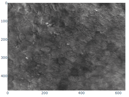
Figure 1:A sample frame from the cilia dataset
While segmentation masks for such a pipeline could be manually generated, the process requires intensive expert labor Doornbos et al., 2021. Requiring manual segmentation before analysis thus greatly increases the barrier to entry for this tool. Not only would it increase the financial strain of adopting ciliary analysis as a clinical tool, but it would also serve as an insurmountable barrier to entry for communities that do not have reliable access to such clinicians in the first place, such as many developing nations and rural populations. Not only can automated segmentation mitigate these barriers to entry, but it can also simplify existing treatment and analysis infrastructure. In particular, it has the potential to reduce the magnitude of work required by an expert clinician, thereby decreasing costs and increasing clinician throughput Quinn et al., 2015Zain et al., 2020. Furthermore, manual segmentation imparts clinician-specific bias which reduces the reproducability of results, making it difficult to verify novel techniques and claims Doornbos et al., 2021.
A thorough review of previous segmentation models, specifically those using the same dataset, shows that current results are poor, impeding tasks further along the pipeline. For this study, model architectures utilize various methods of feature extraction that are hypothesized to improve the accuracy of a base segmentation model, such as using zero-phased PCA maps and Sparse Autoencoder reconstructions with various parameters as a data augmentation tool. Various experiments with these methods provide a summary of both qualitative and quantitative results necessary in ascertaining the viability for such feature extractors to aid in segmentation.
Related Works
Lu et al. (2018) utilized a Dense Net segmentation model as an upstream to a CNN-based Long Short-Term Memory (LSTM) time-series model for classifying cilia based on spatiotemporal patterns. While the model reports good classification accuracy and a high F-1 score, the underlying dataset only contains 75 distinct samples and the results must therefore be taken with great care. Furthermore, Lu et al. (2018) did not report the separate performance of the upstream segmentation network. Their approach did, however, inspire the follow-up methodology of Zain et al. (2020) for segmentation. In particular, they employ a Dense Net segmentation model as well, however they first augment the underlying images with the calculated optical flow. In this way, their segmentation strategy employs both spatial and temporal information. To compare against Lu et al. (2018), the authors evaluated their segmentation model in the same way – as an upstream to an CNN/LSTM classification network. Their model improved the classification accuracy two points above that of Lu et al. (2018). Their reported intersection-over-union (IoU) score is and marks the highest performance achieved on this dataset.
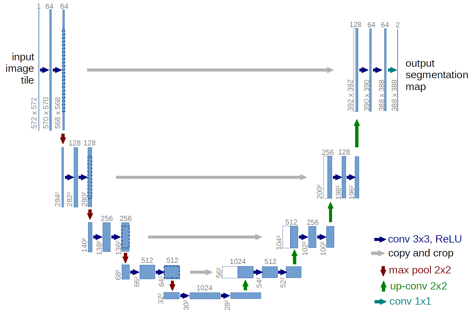
Figure 2:The classical U-Net architecture, which serves as both a baseline and backbone model for this research
One alternative segmentation model, often used in biomedical image processing and analysis, where labelled data sets are relatively small, is the U-Net architecture (Figure 2) Ronneberger et al., 2015. Developed by Ronneberger et al. (2015), U-Nets consist of two parts: contraction and expansion. The contraction path follows the standard strategy of most convolutional neural networks (CNNs), where convolutions are followed by Rectified Linear Unit (ReLU) activation functions and max pooling layers. While max pooling downsamples the images, the convolutions double the number of channels. Upon expansion, up-convolutions are applied to up-sample the image while reducing the number of channels. At each stage, the network concatenates the up-sampled image with the image of corresponding size (cropped to account for border pixels) from a layer in the contracting path. A final layer uses pixel-wise () convolutions to map each pixel to a corresponding class, building a segmentation. Before training, data is generally augmented to provide both invariance in rotation and scale as well as a larger amount of training data. In general, U-Nets have shown high performance on biomedical data sets with low quantities of labelled images, as well as reasonably fast training times on graphics processing units (GPUs) Ronneberger et al., 2015. However, in a few past experiments with cilia data, the U-Net architecture has had low segmentation accuracy Lu et al., 2018. Difficulties modeling cilia with CNN-based architectures include their fine high-variance structure, spatial sparsity, color homogeneity (with respect to the background and ambient cells), as well as inconsistent shape and distribution across samples. Hence, various enhancements to the pure U-Net model are necessary for reliable cilia segmentation.
Methodology
The U-Net architecture is the backbone of the model due to its well-established performance in the biomedical image analysis domain. This paper focuses on extracting and highlighting the underlying features in the image through various means. Therefore, optimization of the U-Net backbone itself is not a major consideration of this project. Indeed, the relative performance of the various modified U-Nets sufficiently communicates the efficacy of the underlying methods. Each feature extraction method will map the underlying raw image to a corresponding feature map. To evaluate the usefulness of these feature maps, the model concatenates these augmentations to the original image and use the aggregate data as input to a U-Net that is slightly modified to accept multiple input channels.
The feature extractors of interest are Zero-phase PCA sphering (ZCA) and a Sparse Autoencoder (SAE), on both of which the following subsections provide more detail. Roughly speaking, these are both lossy, non-bijective transformations which map a single image to a single feature map. In the case of ZCA, empirically the feature maps tend to preserve edges and reduce the rest of the image to arbitrary noise, thereby emphasizing local structure (since cell structure tends not to be well-preserved). The SAE instead acts as a harsh compression and filters out both linear and non-linear features, preserving global structure. Each extractor is evaluated by considering the performance of a U-Net model trained on multi-channel inputs, where the first channel is the original image, and the second and/or third channels are the feature maps extracted by these methods. In particular, the objective is for the doubly-augmented data, or the “composite” model, to achieve state-of-the-art performance on this challenging dataset.
The ZCA implementation utilizes SciPy linear algebra solvers, and both U-Net and SAE architectures use the PyTorch deep learning library. Next, the evaluation stage employs canonical segmentation quality metrics, such as the Jaccard score and Dice coefficient, on various models. When applied to the composite model, these metrics determine any potential improvements to the state-of-the-art for cilia segmentation.
Cilia Data
As in the Zain paper, the input data is a limited set of grayscale cilia imagery, from both healthy patients and those diagnosed with ciliopathies, with corresponding ground truth masks provided by experts. The images are cropped to patches. The images are cropped at random coordinates in order to increase the size and variance of the sample space, and each image is cropped a number of times proportional its resolution. Additionally, crops that contain less than fifteen percent cilia are excluded from the training/test sets. This method increases the size of the training set from 253 images to 1409 images. Finally, standard minmax contrast normalization maps the luminosity to the interval .
Zero-phase PCA sphering (ZCA)
The first augmentation of the underlying data concatenates the input to the backbone U-Net model with the ZCA-transformed data. ZCA maps the underlying data to a version of the data that is “rotated” through the dataspace to ensure certain spectral properties. ZCA in effect can implicitly normalize the data using the most significant (by empirical variance) spatial features present across the dataset. Given a matrix with rows representing samples and columns for each feature, a sphering (or whitening) transformation is one which decorrelates . That is, the covariance of must be equal to the identity matrix. By the spectral theorem, the symmetric matrix – the covariance matrix corresponding to the data, assuming the data is centered – can be decomposed into , where is an orthogonal matrix of eigenvectors and a diagonal matrix of corresponding eigenvalues of the covariance matrix. ZCA uses the sphering matrix and can be thought of as a transformation into the eigenspace of its covariance matrix – projection onto the data’s principal axes, as the minimal projection residual is onto the axes with maximal variance – followed by normalization of variance along every axis and rotation back into the original image space. In order to reduce the amount of two-way correlation in images, Krizhevsky applies ZCA whitening to preprocess CIFAR-10 data before classification and shows that this process nicely preserves features, such as edges Li et al., 2019.
This ZCA implementation uses the Python SciPy library (SciPy), which builds on top of low-level hardware-optimized routines such as BLAS and LAPACK to efficiently calculate many linear algebra operations. In particular, these expirements implement ZCA as a generalized whitening technique. While normal the normal ZCA calculation selects a whitening matrix , a more applicable alternative is where ε is a hyperparameter which attenuates eigenvalue sensitivity. This new “whitening” is actually not a proper whitening since it does not guarantee an identity covariance matrix. It does however serve a similar purpose and actually lends some benefits.
Most importantly, it is indeed a generalization of canonical ZCA. That is to say, recovers canonical ZCA, and provides the spectrum of on the eigenvalues. Otherwise, results in the map . In this case, while all eigenvalues map to smaller values compared to the original map, the smallest eigenvalues map to significantly smaller values compared to the original map. This means that ε serves to “dampen” the effects of whitening for particularly small eigenvalues. This is a valuable feature since often times in image analysis low eigenvalues (and the span of their corresponding eigenvectors) tend to capture high-frequency data. Such data is essential for tasks such as texture analysis, and thus tuning the value of ε helps to preserve this data. ZCA maps for various values of ε on a sample image are shown in Figure 3.
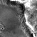 |  |  |  | 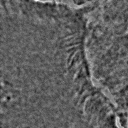 |
Figure 3:Comparison of ZCA maps on a cilia sample image with various levels of ε. The original image is followed by maps with , , , and , from left to right.
Sparse Autoencoder (SAE)
Similar in aim to ZCA, an SAE can augment the underlying images to further filter and reduce noise while allowing the construction and retention of potentially nonlinear spatial features. Autoencoders are deep learning models that first compress data into a low-level latent space and then attempt to reconstruct images from the low-level representation. SAEs in particular add an additional constraint, usually via the loss function, that encourages sparsity (i.e., less activation) in hidden layers of the network. Xu et. al. use the SAE architecture for breast cancer nuclear detection and show that the architecture preserves essential, high-level, and often nonlinear aspects of the initial imagery – even when unlabelled – such as shape and color Xu et al., 2016. An adaptation of the first two terms of their loss function enforces sparsity:
The first term is a standard reconstruction loss (mean squared error), whereas the latter is the mean Kullback-Leibler (KL) divergence between , the activation of a neuron in the encoder, and ρ, the enforced activation. For the case of experiments performed here, remains constant but values of α vary, specifically , , and , for each of which a static dataset is created for feeding into the segmentation model. Larger alpha prioritizes sparsity over reconstruction accuracy, which to an extent, is hypothesized to retain significant low-level features of the cilia. Reconstructions with various values of α are shown in Figure 4
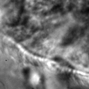 | 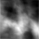 | 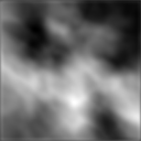 | 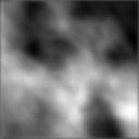 |
Figure 4:Comparison of SAE reconstructions from different training instances with various levels of α (the activation loss weight). From left to right: original image, reconstruction, reconstruction, reconstruction.
A significant amount of freedom can be found in potential architectural choices for SAE. A focus on low-medium complexity models both provides efficiency and minimizes overfitting and artifacts as consequence of degenerate autoencoding. One important danger to be aware of is that SAEs – and indeed, all AEs – are at risk of a degenerate solution wherein a sufficiently complex decoder essentially learns to become a hashmap of arbitrary (and potentially random) encodings.
The SAE will therefore utilize a CNN architecture, as opposed to more modern transformer-style architectures, since the simplicity and induced spatial bias provide potent defenses against overfitting and mode collapse. Furthermore the encoder will use Spatial Broadcast Decoding (SBD) which provides a method for decoding from a latent vector using size-preserving convolutions, thereby preserving the spatial bias even in decoding, and eliminating the artifacts generated by alternate decoding strategies such as “transposed” convolutions Watters et al., 2019.
Spatial Broadcast Decoding (SBD)
Spatial Broadcast Decoding provides an alternative method from ”transposed” (or ”skip”) convolutions to upsample images in the decoder portion of CNN-based autoencoders. Rather than maintaining the square shape, and hence associated spatial properties, of the latent representation, the output of the encoder is reshaped into a single one-dimensional tensor per input image, which is then tiled to the shape of the desired image (in this case, ). In this way, the initial dimension of the latent vector becomes the number of input channels when fed into the decoder, and two additional channels are added to represent 2-dimensional spatial coordinates. In its initial publication, SBD has been shown to provide effective results in disentangling latent space representations in various autoencoder models.
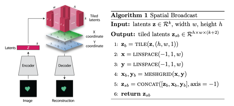
Figure 5:Illustration and pseudocode for Spatial Broadcast Decoding Watters et al., 2019
U-Net
All models use a standard U-Net and undergo the same training process to provide a solid basis for analysis. Besides the number of input channels to the initial model (1 plus the number of augmentation channels from SAE and ZCA, up to 3 total channels), the model architecture is identical for all runs. A single-channel (original image) U-Net first trains as a basis point for analysis. The model trains on two-channel inputs provided by ZCA (original image concatenated with the ZCA-mapped one) with various ε values for the dataset, and similarly SAE with various α values, train the model. Finally, composite models train with a few combinations of ZCA and SAE hyperparameters. Each training process uses binary cross entropy loss with a learning rate of for 225 epochs.
Results
Figure 6, Figure 7, Figure 8, and Figure 9 show masks produced on validation data from instances of the four model types. While the former three show results near the end of training (about 200-250 epochs), Figure 9 was taken only 10 epochs into the training process. Notably, this model, the composite pipeline, produced usable artifacts in mere minutes of training, whereas other models did not produce similar results until after about 10-40 epochs.
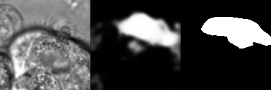
Figure 6:Artifacts generated during the training of U-Net. From left to right: original image, generated segmentation mask (pre-threshold), ground-truth segmentation mask

Figure 7:Artifacts generated during the training of ZCA+U-Net. From left to right: original image, ZCA-mapped image, generated segmentation mask (pre-threshold), ground-truth segmentation mask

Figure 8:Artifacts generated during the training of SAE+U-Net. From left to right: original image, SAE-reconstructed image, generated segmentation mask (pre-threshold), ground-truth segmentation mask

Figure 9:Artifacts generated 10 epochs into the training of the composite U-Net. From left to right: original image, ZCA-mapped image, SAE-mapped image, generated segmentation mask (pre-threshold), ground-truth segmentation mask
Figure 10 provides a summary of experiments performed with and augmented data, along with a few composite models and a base U-Net for comparison. These models were produced with data augmentation at various values of α (for the Sparse Autoencoder loss function) and ε (for ZCA) discussed above. While the table provides five metrics, those of primary importance are the Intersection over Union (IoU), or Jaccard Score, as well as the Dice (or F1) score, which are the most commonly used metrics for evaluating the performance of segmentation models. Most feature extraction models at least marginally improve the performance in of the U-Net in terms of IoU and Dice scores, and the best-performing composite model (with ε of for ZCA and α of for SAE) provide an improvement of approximately from the base U-Net in these metrics. There does not seem to be an obvious correlation between which feature extraction hyperparameters provided the best performance for individual ZCA+U-Net and SAE+U-Net models versus those for the composite pipeline, but further experiments may assist in analyzing this possibility.
| Extractor Parameters | Scores | ||||||
| Model | ε (ZCA) | α (SAE) | IoU | Accuracy | Recall | Dice | Precision |
| U-Net (base) | — | — | 0.399 | 0.759 | 0.501 | 0.529 | 0.692 |
| ZCA + U-Net | — | 0.395 | 0.754 | 0.509 | 0.513 | 0.625 | |
| — | 0.401 | 0.732 | 0.563 | 0.539 | 0.607 | ||
| — | 0.408 | 0.756 | 0.543 | 0.546 | 0.644 | ||
| — | 0.419 | 0.758 | 0.563 | 0.557 | 0.639 | ||
| SAE + U-Net | — | 0.380 | 0.719 | 0.568 | 0.520 | 0.558 | |
| — | 0.398 | 0.751 | 0.512 | 0.526 | 0.656 | ||
| — | 0.416 | 0.735 | 0.607 | 0.555 | 0.603 | ||
| Composite | 0.401 | 0.761 | 0.506 | 0.521 | 0.649 | ||
| 0.441 | 0.767 | 0.580 | 0.585 | 0.661 | |||
| 0.305 | 0.722 | 0.398 | 0.424 | 0.588 | |||
| 0.392 | 0.707 | 0.624 | 0.530 | 0.534 | |||
| 0.413 | 0.770 | 0.514 | 0.546 | 0.678 | |||
| 0.413 | 0.751 | 0.565 | 0.550 | 0.619 | |||
| 0.392 | 0.719 | 0.602 | 0.527 | 0.571 | |||
| 0.395 | 0.759 | 0.480 | 0.521 | 0.711 | |||
| 0.405 | 0.729 | 0.587 | 0.545 | 0.591 | |||
| 0.383 | 0.753 | 0.487 | 0.503 | 0.655 | |||
| 0.380 | 0.736 | 0.526 | 0.519 | 0.605 | |||
| 0.293 | 0.674 | 0.445 | 0.418 | 0.487 | |||
Figure 10:A summary of segmentation scores on test data for a base U-Net model, ZCA+U-Net, SAE+U-Net, and a composite model, with various feature extraction hyperparameters. The best result for each scoring metric is in bold.
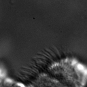
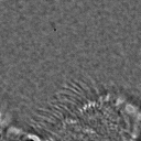
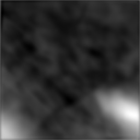
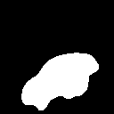
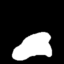
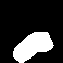
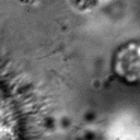
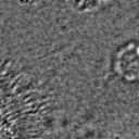
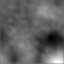
The base U-Net does outperform the others in precision, however. Analysis of predicted masks from various models, some of which are shown in Figure 11, shows that the base U-Net model tends to under-predict cilia, explaining the relatively high precision. Previous endeavors in cilia segmentation also revealed this pattern.
| Input Images | Predicted Masks | ||||||
| Original | ZCA | SAE | Ground Truth | Base U-Net | ZCA + U-Net | SAE + U-Net | Composite |
 |  |  |  |  |  |  |  |
 |  |  |  |  |  |  |  |
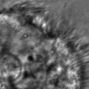 | 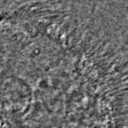 | 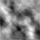 |  |  |  |  |  |
Figure 11:Comparison of predicted masks and ground truth for three test images. ZCA mapped images with and SAE reconstructions with are used where applicable.
Conclusions
This paper highlights the current shortcomings of automated, deep-learning based segmentation models for cilia, specifically on the data provided to the Quinn Research Group, and provides two additional methods, Zero-Phase PCA Sphering (ZCA) and Sparse Autoencoders (SAE), for performing feature extracting augmentations with the purpose of aiding a U-Net model in segmentation. An analysis of U-Nets with various combinations of these feature extraction and parameters help determine the feasibility for low-level feature extraction in improving cilia segmentation, and results from initial experiments show up to increases in relevant metrics.
While these improvements, in general, have been marginal, these results show that pre-segmentation based feature extraction methods, particularly the avenues explored, provide a worthwhile path of exploration and research for improving cilia segmentation. Implications internal to other projects within the research group sponsoring this research are clear. As discussed earlier, later pipelines of ciliary representation and modeling are currently being bottlenecked by the poor segmentation masks produced by base U-Nets, and the under-segmented predictions provided by the original model limits the scope of what these later stages may achieve. Better predictions hence tend to transfer to better downstream results.
These results also have significant implications outside of the specific task of cilia segmentation and modeling. The inherent problem that motivated an introduction of feature extraction into the segmentation process was the poor quality of the given dataset. From occlusion to poor lighting to blurred images, these are problems that typically plague segmentation models in the real world, where data sets are not of ideal quality. For many modern computer vision tasks, segmentation is a necessary technique to begin analysis of certain objects in an image, including any forms of objects from people to vehicles to landscapes. Many images for these tasks are likely to come from low-resolution imagery, whether that be satellite data or security cameras, and are likely to face similar problems as the given cilia dataset in terms of image quality. Even if this is not the case, manual labelling, like that of this dataset and convenient in many other instances, is prone to error and is likely to bottleneck results. As experiments have shown, feature extraction through SAE and ZCA maps are a potential avenue for improvement of such models and would be an interesting topic to explore on other problematic datsets.
Especially compelling, aside from the raw numeric results, is how soon composite pipelines began to produce usable masks on training data. As discussed earlier, most original U-Net models would take at least 40-50 epochs before showing any accurate predictions on training data. However, when feeding in composite SAE and ZCA data along with the original image, unusually accurate masks were produced within just a couple minutes, with usable results at 10 epochs. This has potential implications in scenarios such as one-shot and/or unsupervised learning, where models cannot train over a large datset.
Future Research
While this work establishes a primary direction and a novel perspective for segmenting cilia, there are many interesting and valuable directions for future planned research. In particular, a novel and still-developing alternative to the convolution layer known as a Sharpened Cosine Similarity (SCS) layer has begun to attract some attention. While regular CNNs are proficient at filtering, developing invariance to certain forms of noise and perturbation, they are notoriously poor at serving as a spatial indicator for features. Convolution activations can be high due to changes in luminosity and do not necessarily imply the distribution of the underlying luminosity, therefore losing precise spatial information. By design, SCS avoids these faults by considering the mathematical case of a “normalized” convolution, wherein neither the magnitude of the input, nor of the kernel, affect the final output. Instead, SCS activations are dictated purely by the relative magnitudes of weights in the kernel, which is to say by the spatial distribution of features in the input Pisonir, 2022. Domain knowledge suggests that cilia, while able to vary greatly, all share relatively unique spatial distributions when compared to non-cilia such as cells, out-of-phase structures, microscopy artifacts, etc. Therefore, SCS may provide a strong augmentation to the backbone U-Net model by acting as an additional layer in tandem with the already existing convolution layers. This way, the model is a true generalization of the canonical U-Net and is less likely to suffer poor performance due to the introduction of SCS.
Another avenue of exploration would be a more robust ablation study on some of the hyperparameters of the feature extractors used. While most of the hyperparameters were chosen based on either canonical choices Xu et al., 2016 or through empirical study (e.g. ε for ZCA whitening), a more comprehensive hyperparameter search would be worth consideration. This would be especially valuable for the composite model since the choice of most optimal hyperparameters is dependent on the downstream tasks and therefore may be different for the composite model than what was found for the individual models.
More robust data augmentation could additionally improve results. Image cropping and basic augmentation methods alone provided minor improvements of just the base U-Net from the state of the art. Regarding the cropping method, an upper threshold for the percent of cilia per image may be worth implementing, as cropped images containing over approximately cilia produced poor results, likely due to a lack of surrounding context. Additionally, rotations and lighting/contrast adjustments could further augment the data set during the training process.
Re-segmenting the cilia images by hand, a planned endeavor, will likely provide more accurate masks for the training process. This is an especially difficult task for the cilia dataset, as the poor lighting and focus even causes medical professionals to disagree on the exact location of cilia in certain instances. However, the research group associated with this paper is currently in the process of setting up a web interface for such professionals to ”vote” on segmentation masks. Additionally, it is likely worth experimenting with various thresholds for converting U-Net outputs into masks, and potentially some form of region growing to dynamically aid the process.
Finally, it is possible to train the SAE and U-Net jointly as an end-to-end system. Current experimentation has foregone this path due to the additional computational and memory complexity and has instead opted for separate training to at least justify this direction of exploration. Training in an end-to-end fashion could lead to a more optimal result and potentially even an interesting latent representation of ciliary features in the image. It is worth noting that larger end-to-end systems like this tend to be more difficult to train and balance, and such architectures can fall into degenerate solutions more readily.
Copyright © 2022 Zain et al. This is an open-access article distributed under the terms of the Creative Commons Attribution 3.0 Unported license.
- CNN
- convolutional neural network
- GPU
- graphics processing unit
- IoU
- intersection-over-union
- KL
- Kullback-Leibler
- LSTM
- Long Short-Term Memory
- ReLU
- Rectified Linear Unit
- SAE
- Sparse Autoencoder
- SBD
- Spatial Broadcast Decoding
- SCS
- Sharpened Cosine Similarity
- ZCA
- Zero-phase PCA sphering
- Li, F., Wang, C., Liu, X., Peng, Y., & Jin, S. (2018). A composite model of wound segmentation based on traditional methods and deep neural networks. Computational Intelligence and Neuroscience, 2018. 10.1155/2018/4149103
- Quinn, S. P., Zahid, M. J., Durkin, J. R., Francis, R. J., Lo, C. W., & Chennubhotla, S. C. (2015). Automated identification of abnormal respiratory ciliary motion in nasal biopsies. Science Translational Medicine, 7(299), 299ra124 |-| 299ra124. 10.1126/scitranslmed.aaa1233
- Ishikawa, T. (2017). Axoneme structure from motile cilia. Cold Spring Harbor Perspectives in Biology, 9(1), a028076. 10.1101/cshperspect.a028076
- Zain, M., Rao, S., Safir, N., Wyner, Q., Humphrey, I., Eldridge, A., Li, C., AlAila, B., & Quinn, S. (2020). Towards an Unsupervised Spatiotemporal Representation of Cilia Video Using A Modular Generative Pipeline. Proceedings of the Python in Science Conference. 10.25080/majora-342d178e-017
- Doornbos, C., van Beek, R., Bongers, E. M., Lugtenberg, D., Klaren, P., Vissers, L. E., Roepman, R., Oud, M. M., & others. (2021). Cell-based assay for ciliopathy patients to improve accurate diagnosis using ALPACA. European Journal of Human Genetics, 29(11), 1677 |-| 1689. 10.1038/s41431-021-00907-9
- Lu, C., Marx, M., Zahid, M., Lo, C. W., Chennubhotla, C., & Quinn, S. P. (2018). Stacked Neural Networks for end-to-end ciliary motion analysis. CoRR. 10.48550/arXiv.1803.07534
- Ronneberger, O., Fischer, P., & Brox, T. (2015). U-Net: Convolutional Networks for Biomedical Image Segmentation. CoRR. 10.48550/arXiv.1505.04597
- Li, H., jun Xiao-Wu, & Durrani, T. S. (2019). Infrared and visible image fusion with ResNet and zero-phase component analysis. Infrared Physics & Technology, 102, 103039. https://doi.org/10.1016/j.infrared.2019.103039
- Xu, J., Xiang, L., Liu, Q., Gilmore, H., Wu, J., Tang, J., & Madabhushi, A. (2016). Stacked Sparse Autoencoder (SSAE) for Nuclei Detection on Breast Cancer Histopathology Images. IEEE Transactions on Medical Imaging, 35(1), 119–130. 10.1109/TMI.2015.2458702
- Watters, N., Matthey, L., Burgess, C. P., & Lerchner, A. (2019). Spatial Broadcast Decoder: A Simple Architecture for Learning Disentangled Representations in VAEs. CoRR. 10.48550/arXiv.1901.07017
- Pisonir, R. (2022). Sharpened Cosine Distance as an Alternative for Convolutions. In rpisoni.dev. https://www.rpisoni.dev
