multinterp
A Unified Interface for Multivariate Interpolation in the Scientific Python Ecosystem
Abstract
Multivariate interpolation is a fundamental tool in scientific computing used to approximate the values of a function between known data points in multiple dimensions. Despite its importance, the Python ecosystem offers a fragmented landscape of specialized tools for this task. This fragmentation hinders code reusability, experimentation, and efficient deployment across diverse hardware. The multinterp package was developed to address this challenge. It provides a unified interface for various grids used for interpolation (regular, irregular, and curvilinear), supports multiple backends (CPU, parallel, and GPU), and includes tools for multivalued interpolation and interpolation of derivatives. This paper introduces multinterp, demonstrates its capabilities, and invites the community to contribute to its development.
1Introduction
In scientific computing, interpolation is a fundamental method used to approximate new data points within a range of known functional data points. When this concept is applied to functions with multiple variables, it is known as multivariate interpolation. This technique is crucial for various scientific applications, including data analysis, numerical modeling, and visualizing complex datasets.
Over time, the scientific Python ecosystem has developed various specialized tools for multivariate interpolation. These powerful tools are spread across different packages, each designed for specific purposes and for distinct data types. This scattering of tools across multiple packages creates challenges for researchers and practitioners.
One major issue is the inconsistency of interfaces across different packages. The varying syntax and usage patterns make it difficult for users to switch between interpolation methods or compare their performance effectively. Additionally, many existing tools are designed for CPU-only execution, lacking GPU acceleration or parallel processing support. This limitation can significantly impact performance, especially when dealing with large datasets or complex interpolation tasks.
Another challenge stems from the restricted functionality of some packages. Certain tools focus solely on specific types of interpolation, such as those for structured data, while lacking support for advanced features like multivalued interpolation or derivative calculations. This specialization often forces researchers to use multiple packages to cover all their interpolation needs, leading to an inefficient workflow. The need to learn and integrate various packages increases development time and introduces potential inconsistencies in the codebase.
The multinterp package was developed to address these challenges to provide a comprehensive framework for multivariate interpolation in python with several key features. It offers a unified interface for various interpolation grids, including regular (rectilinear), irregular (unstructured), and curvilinear grids, allowing users to easily switch between different grid types without changing their code structure.
Furthermore, multinterp supports multiple backends, including CPU (using numpy and scipy), parallel processing (using numba), and GPU acceleration (using cupy, pytorch, and jax). This flexibility enables users to optimize performance based on their available computational resources. The package also includes tools for multivalued interpolation and interpolation of derivatives, expanding its utility for a wide range of scientific applications.
Perhaps most importantly, multinterp provides a consistent API that allows easy switching between different interpolation methods and backends. This feature simplifies code development and facilitates experimentation with various interpolation techniques and performance optimization strategies.
In the following sections, we will introduce the main concepts of grid interpolation, demonstrate the capabilities of multinterp for different types of grids, and compare its performance with existing tools. We will conclude by discussing the project’s current state and inviting community contributions to further development.
2Background and Concepts
Before diving into the specifics of multinterp, it is crucial to understand some fundamental concepts in multivariate interpolation and the challenges they present.
2.1Interpolation Basics
At its core, interpolation is about approximating functional values between known data points. This might involve drawing a line or curve between points in one dimension. The process becomes more complex in multiple dimensions, involving surfaces or hypersurfaces.
2.2Grid Types
The arrangement of known data points, called the grid, significantly influences the choice of interpolation method and its computational efficiency. In multinterp, we consider three main types of grids:
Rectilinear Grids: These are the simplest and most common. Data points form a regular pattern along each dimension, though the spacing between points may vary. Moreover, these grids can be represented by the cross product of 1-dimensional vectors, making them easy to work with.
Curvilinear Grids: These maintain a structured relationship between neighboring points, but the grid lines may be curved or warped. Their main advantage is that these grids are monotonic in each coordinate dimension, allowing for an easy and efficient transformation into a rectilinear grid.
Unstructured Grids: These have irregularly spaced data points with no inherent structure. They are often encountered in experimental data collection or adaptive numerical methods. Interpolation on unstructured grids is more challenging and requires more sophisticated algorithms.
Table 1:Grids and structures implemented in “multinterp”.
| Grid | Structure | Geometry |
|---|---|---|
| Rectilinear | Regular | Rectangular mesh |
| Curvilinear | Regular | Quadrilateral mesh |
| Unstructured | Irregular | Random |
2.3Existing Interpolation Methods
Various methods exist for interpolation, each with its strengths and limitations:
- Nearest Neighbor: Assigns the value of the nearest known point or a weighted average of the nearest few points. Simple but can be inaccurate.
- Linear/Multilinear: Assumes a linear relationship between points. Fast but can miss complex patterns.
- Polynomial: Higher-order polynomials are used to fit the data. It can capture more complex relationships but may oscillate between points.
- Spline: Uses piecewise polynomials. Offers a balance between smoothness and accuracy.
- Radial Basis Function (RBF): Uses a sum of radially symmetric functions. Useful for scattered data.
Each of these methods may be implemented differently for different grid types, leading to the fragmentation in the Python ecosystem that multinterp aims to address. multinterp currently mainly implements multilinear interpolation and aims to add more methods and grid types in the future.
3The multinterp Package
The multinterp package is a unified framework for multivariate interpolation in python, designed to address the challenges outlined in the previous sections. It offers several key features:
Unified Interface: A consistent API for interpolation, regardless of data structure or desired backend, reducing the learning curve and promoting code reusability. This consistency extends across different grid types (rectilinear, curvilinear, and unstructured), allowing users to switch between grid types with minimal code changes.
Hardware Adaptability: Seamless support for CPU (
numpy,scipy), parallel (numba), and GPU (cupy,pytorch,jax) backends, empowering users to optimize performance based on their computational resources.Broad Functionality: Tools for regular/rectilinear interpolation, multivalued interpolation, and derivative calculations, addressing a wide range of scientific problems.
The multinterp package offers several advantages over existing tools:
Flexibility: Unlike specialized packages that focus on specific grid types or interpolation methods,
multinterpprovides a unified framework that can handle various grid types and interpolation scenarios.Performance: By supporting multiple backends, including GPU acceleration,
multinterpcan offer significant performance improvements over CPU-only implementations, especially for large datasets. Our benchmarks show up to 10x speedup for large 3D grids when using GPU backends.Ease of Use: The consistent API across different grid types and backends simplifies the learning curve and makes it easier for users to experiment with different approaches. For instance, switching from CPU to GPU interpolation often requires changing a single parameter.
Currently, multinterp primarily implements multilinear interpolation, which balances simplicity, speed, and accuracy for many applications. This method is particularly efficient for rectilinear grids. The core implementation uses efficient numpy operations for fast computation.
However, we recognize the limitations of multilinear interpolation, such as its inability to capture complex, non-linear relationships in the data. Future development plans include implementing additional interpolation methods such as polynomial, spline, and radial basis function interpolation. These methods can offer improved accuracy for certain types of data, albeit at the cost of increased computational complexity.
The multinterp package is currently in its beta stage, but it offers a strong foundation and welcomes community contributions to reach its full potential. We invite collaboration to improve documentation, expand the test suite, and ensure the codebase aligns with the highest standards of Python package development.
4Rectilinear Interpolation
Rectilinear grids are the foundation of many scientific computing applications. They are simple yet powerful, allowing for efficient data representation and manipulation. In a rectilinear grid, data points form a regular pattern along each dimension, though the spacing between points may vary.
4.1The Basics of Rectilinear Grids
A rectilinear grid in 2D can be thought of as a sheet of graph paper where the lines might not be evenly spaced. In 3D, you can imagine a stack of these sheets, again with potentially varying spacing between them. Mathematically, we can represent a 2D rectilinear grid using two 1D arrays of increasing values:
where and for all . The full grid is then represented by the tensor product , resulting in dimensions .
This structure allows for efficient interpolation algorithms, as we can quickly locate the nearest known values to predict the function’s behavior in unknown spaces. This is because we only need to search each dimension once and independently of the other.
Figure 1:Transformation between non-uniform and uniform rectilinear grids. This process is critical to efficient interpolation on rectilinear grids.
4.2Multilinear Interpolation with multinterp
The multinterp package provides a straightforward yet powerful implementation of multilinear interpolation. It supports various backends, including numpy, scipy, numba, cupy, pytorch, and jax, allowing users to choose the most suitable option for their computational environment.
At the heart of multinterp’s rectilinear interpolation is the map_coordinates function from scipy.ndimage. This function is versatile, taking an array of input values and an array of coordinates and returning interpolated values at those coordinates. Here is how it works:
- The
inputarray contains known values on a coordinate (index) grid. For example,input[i,j,k]is the known value at coordinate(i,j,k). - The
coordinatesarray contains fractional coordinates where we want to interpolate. For instance,coordinates[0] = (1.5, 2.3, 3.1)indicates we want to interpolate at a point between integer grid coordinates.
However, real-world functions are often not defined on a simple coordinate grid. This is where multinterp’s get_coordinates function comes in. It maps the functional input grid (defined on real numbers) and the coordinate grid (defined on non-negative integers).
Let us look at a practical example to see how this works:
import `numpy` as np
from multinterp import MultivariateInterp

# Define a function to interpolate
def squared_coords(x, y):
    return x**2 + y**2

# Create a non-uniform rectilinear grid
x_grid = np.geomspace(1, 11, 11) - 1
y_grid = np.geomspace(1, 11, 11) - 1
x_mat, y_mat = np.meshgrid(x_grid, y_grid, indexing="ij")

# Evaluate the function on this grid
z_mat = squared_coords(x_mat, y_mat)

# Create the interpolator
interp = MultivariateInterp(z_mat, [x_grid, y_grid])

# Define points for interpolation
x_new, y_new = np.meshgrid(
 np.linspace(0, 10, 11),
 np.linspace(0, 10, 11),
    indexing="ij",
)

# Perform interpolation
z_interp = interp(x_new, y_new)
In this example, we use a squared coordinates function (x^2+y^2) as our test case. This function is chosen because it produces a simple curved surface in 3D, making it easy to verify the interpolation results visually. We create a non-uniform grid using geomspace, which gives us more points near the origin and fewer points farther out. This non-uniform grid demonstrates multinterp’s ability to handle varying grid spacings effectively.
The MultivariateInterp class encapsulates the interpolation process, making it easy to create an interpolator and apply it to new points. This object-oriented approach allows for easy reuse and chaining of operations, as seen in the next section on derivatives.
4.3Derivatives
The multinterp package also allows calculating derivatives of the interpolated function defined on a rectilinear grid. This is done by using the function get_grad, which wraps numpy’s gradient function to calculate the gradient of the interpolated function at the given coordinates.
Consider the following function along with its analytical derivatives:
def trig_func(x, y):
    return y * np.sin(x) + x * np.cos(y)


def trig_func_dx(x, y):
    return y * np.cos(x) + np.cos(y)


def trig_func_dy(x, y):
    return np.sin(x) - x * np.sin(y)
First, we create a sample input gradient and evaluate the function at those points. Notice that we are not using the analytical derivatives to create the interpolation function. Instead, we will use these to compare the results of the numerical derivatives.
x_grid = np.geomspace(1, 11, 1000) - 1
y_grid = np.geomspace(1, 11, 1000) - 1
x_mat, y_mat = np.meshgrid(x_grid, y_grid, indexing="ij")

z_mat = trig_func(x_mat, y_mat)
Now, we generate a different grid, which will be used as our query points.
x_new, y_new = np.meshgrid(
 np.linspace(0, 10, 1000),
 np.linspace(0, 10, 1000),
    indexing="ij",
)
Then, we can compare our interpolation function with the analytical function and see that these are very close to each other.
mult_interp = MultivariateInterp(z_mat, [x_grid, y_grid], backend="cupy")
z_mult_interp = mult_interp(x_new, y_new).get()
z_true = trig_func(x_new, y_new)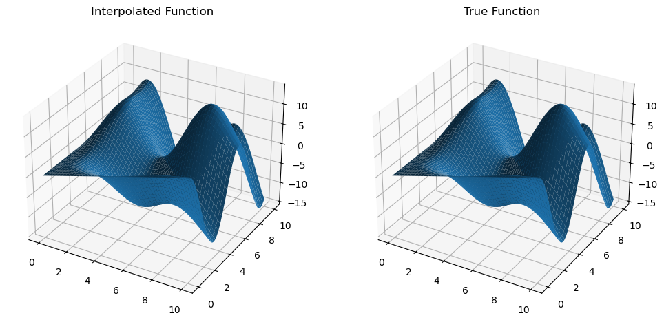
We can use the method .diff(argnum) of MultivariateInterp to evaluate numerical derivatives, which provides an object-oriented way to compute gradients. For example, calling mult_interp.diff(0) returns a MultivariateInterp object that represents the numerical derivative of the function with respect to the first argument on the same input grid.
We can now compare the numerical and analytical derivatives and see that these are indeed very close to each other.
dfdx = mult_interp.diff(0)
z_dfdx = dfdx(x_new, y_new).get()
dfdx_true = trig_func_dx(x_new, y_new)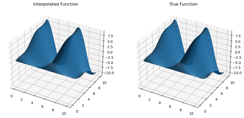
Similarly, we can compute the derivatives with respect to the second argument and see that they produce an accurate result.
dfdy = mult_interp.diff(1)
z_dfdy = dfdy(x_new, y_new).get()
dfdy_true = trig_func_dy(x_new, y_new)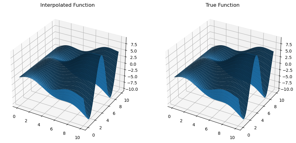
The choice of returning object-oriented interpolation functions for the numerical derivatives is beneficial, as it allows for reusability without re-computation and easy chaining of operations. For example, we can compute the function’s second derivative with respect to the first argument by calling mult_interp.diff(0).diff(0).
4.4Multivalued Interpolation
Finally, the multinterp package allows for multivalued interpolation on rectilinear grids via the MultivaluedInterp class.
Consider the following multivalued function:
def squared_coords(x, y):
    return x**2 + y**2


def trig_func(x, y):
    return y * np.sin(x) + x * np.cos(y)


def multivalued_func(x, y):
    return np.array([squared_coords(x, y), trig_func(x, y)])
As before, we can generate values on a sample input grid and create a grid of query points.
x_grid = np.geomspace(1, 11, 1000) - 1
y_grid = np.geomspace(1, 11, 1000) - 1
x_mat, y_mat = np.meshgrid(x_grid, y_grid, indexing="ij")

z_mat = multivalued_func(x_mat, y_mat)

x_new, y_new = np.meshgrid(
 np.linspace(0, 10, 1000),
 np.linspace(0, 10, 1000),
    indexing="ij",
)
MultivaluedInterp can easily interpolate the function at the query points and avoid repeated calculations.
from multinterp.rectilinear._multi import MultivaluedInterp

mult_interp = MultivaluedInterp(z_mat, [x_grid, y_grid], backend="cupy")
z_mult_interp = mult_interp(x_new, y_new).get()
z_true = multivalued_func(x_new, y_new)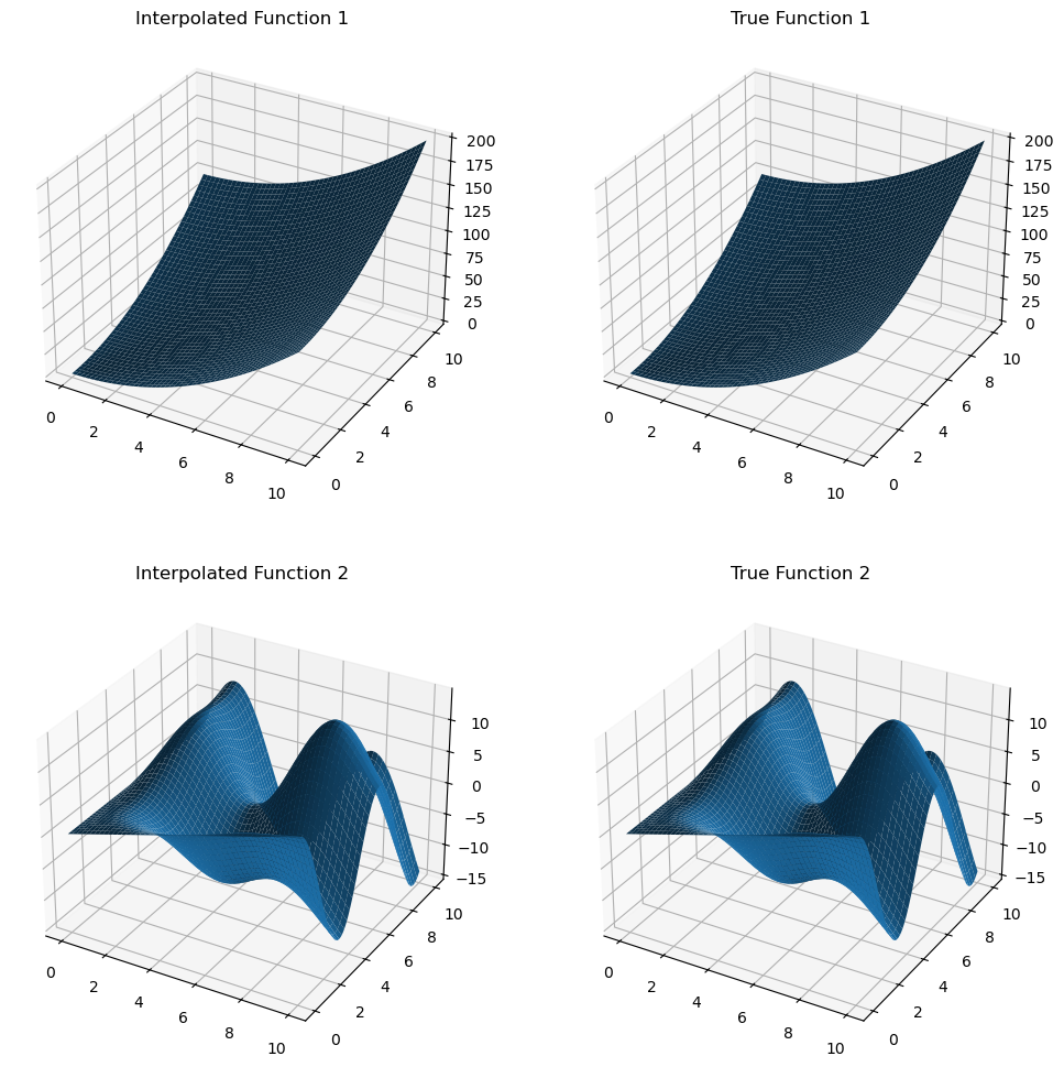
5Curvilinear Interpolation
A curvilinear grid is a regular grid whose input coordinates are curved or warped in some regular way. However, simple transformations can nevertheless transform it into a regular grid. That is, every quadrangle in the grid can be transformed into a rectangle by remapping its vertices. There are two approaches to curvilinear interpolation in multinterp: the first requires a “point location” algorithm to determine which quadrangle the input point lies in, and the second requires a “dimensional reduction” algorithm to generate an interpolated value from the known values in the quadrangle.
Figure 2:A curvilinear grid can be transformed into a rectilinear grid by simply remapping its vertices.
Suppose we have a collection of values for an unknown function and their respective coordinate points. For illustration, assume the values come from the following function:
def function_1(x, y):
    return x * (1 - x) * np.cos(4 * np.pi * x) * np.sin(4 * np.pi * y**2) ** 2
The points are randomly scattered in the unit square and have no regular structure. This is achieved by randomly shifting a well-structured grid at every point.
rng = np.random.default_rng(0)
warp_factor = 0.01
x_list = np.linspace(0, 1, 20)
y_list = np.linspace(0, 1, 20)
x_temp, y_temp = np.meshgrid(x_list, y_list, indexing="ij")
rand_x = x_temp + warp_factor * (rng.random((x_list.size, y_list.size)) - 0.5)
rand_y = y_temp + warp_factor * (rng.random((x_list.size, y_list.size)) - 0.5)
values = function_1(rand_x, rand_y)
Suppose we want to interpolate this function on a rectilinear grid, a process called “regridding.”
grid_x, grid_y = np.meshgrid(
 np.linspace(0, 1, 100),
 np.linspace(0, 1, 100),
    indexing="ij",
)
We use multinterp’s Warped2DInterp and Curvilinear2DInterp classes to do this. The class takes the following arguments:
values: an ND-array of values for the function at the pointsgrids: a list of ND-arrays of coordinates for the pointsbackend: the backend to use for interpolation currently onlyscipyandnumbaare supported forWarped2DInterp, and onlyscipyis supported forCurvilinear2DInterpfor now.
from multinterp.curvilinear import Curvilinear2DInterp, Warped2DInterp

warped_interp = Warped2DInterp(values, (rand_x, rand_y), backend="numba")
warped_interp.warmup()
Once we create the interpolator objects, we can evaluate the functions on the query grids and compare their time performance.
start = time()
warped_grid = warped_interp(grid_x, grid_y)
print(f"Warped interpolation took {time() - start:.5f} seconds")
curvilinear_interp = Curvilinear2DInterp(values, (rand_x, rand_y))
start = time()
curvilinear_grid = curvilinear_interp(grid_x, grid_y)
print(f"Curvilinear interpolation took {time() - start:.5f} seconds")Now, we can compare the interpolation results with the original function. Below, we plot the original function and the known sample points. Notice that the points are almost rectilinear but have been randomly shifted to create a more challenging interpolation problem.
plt.imshow(function_1(grid_x, grid_y).T, extent=(0, 1, 0, 1), origin="lower")
plt.plot(rand_x.flat, rand_y.flat, "ok", ms=2, label="input points")
plt.title("Original")
plt.legend(loc="lower right")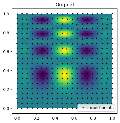
Then, we can look at the result for each interpolation method and compare it to the original function.
fig, axs = plt.subplots(1, 3, figsize=(9, 6))
titles = ["Original", "WarpedInterp", "CurvilinearInterp"]
grids = [function_1(grid_x, grid_y), warped_grid, curvilinear_grid]

for ax, title, grid in zip(axs.flat, titles, grids):
    im = ax.imshow(grid.T, extent=(0, 1, 0, 1), origin="lower")
    ax.set_title(title)

plt.tight_layout()
plt.show()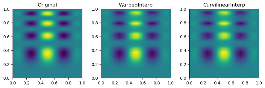
In short, multinterp’s Warped2DInterp and Curvilinear2DInterp classes are helpful for interpolating functions on curvilinear grids with a quadrilateral structure but are not perfectly rectangular.
6Unstructured Interpolation
Figure 3:Unstructured grids are irregular and often require a triangulation step, which might be computationally expensive and time-consuming.
Suppose we have a collection of values for an unknown function and their respective coordinate points. For illustration, assume the values come from the following function:
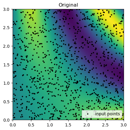
def function_1(u, v):
    return u * np.cos(u * v) + v * np.sin(u * v)
The points are randomly scattered within a square and have no regular structure.
rng = np.random.default_rng(0)
rand_x, rand_y = rng.random((2, 1000)) * 3
values = function_1(rand_x, rand_y)
Suppose we want to interpolate this function on a rectilinear grid.
grid_x, grid_y = np.meshgrid(
 np.linspace(0, 3, 100),
 np.linspace(0, 3, 100),
    indexing="ij",
)
We use multinterp’s UnstructuredInterp class to do this. The class takes the following arguments:
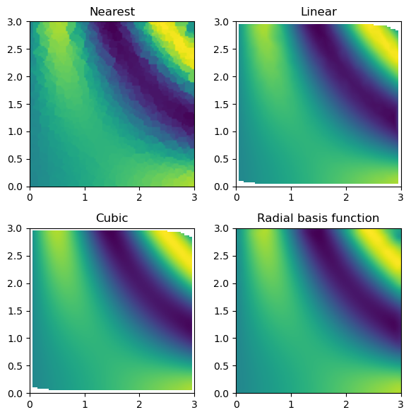
values: an ND-array of values for the function at the pointsgrids: a list of ND-arrays of coordinates for the pointsmethod: the interpolation method to use, with options “nearest”, “linear”, “cubic” (for 2D only), and “rbf”. The default is'linear'.
The UnstructuredInterp class is an object-oriented wrapper around scipy.interpolate’s functions for multivariate interpolation on unstructured data, which are NearestNDInterpolator, LinearNDInterpolator, CloughTocher2DInterpolator, and RBFInterpolator. The advantage of using multinterp’s UnstructuredInterp class is that it provides a consistent interface for all these methods, making it easier to switch between them and other interpolators in the multinterp package.
nearest_interp = UnstructuredInterp(values, (rand_x, rand_y), method="nearest")
linear_interp = UnstructuredInterp(values, (rand_x, rand_y), method="linear")
cubic_interp = UnstructuredInterp(values, (rand_x, rand_y), method="cubic")
rbf_interp = UnstructuredInterp(values, (rand_x, rand_y), method="rbf")
Once we create the interpolator objects, we can use them using the __call__ method, which takes as many arguments as there are dimensions.
nearest_grid = nearest_interp(grid_x, grid_y)
linear_grid = linear_interp(grid_x, grid_y)
cubic_grid = cubic_interp(grid_x, grid_y)
rbf_grid = rbf_interp(grid_x, grid_y)
Now, we can compare the interpolation results with the original function. Below, we plot the original function and the known sample points.
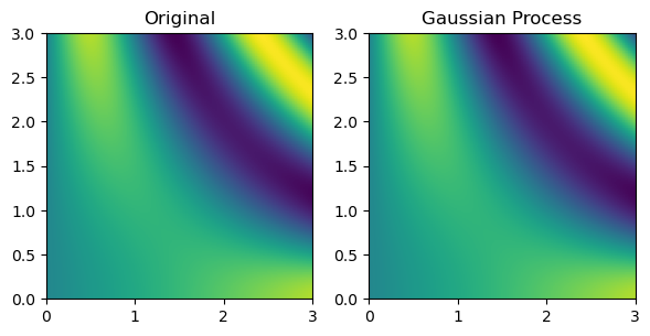
Then, we can look at the result for each interpolation method and compare it to the original function.
Finally, multinterp also provides a set of interpolators organized around the concept of regression. As a demonstration, below, we use a RegressionUnstructuredInterp interpolator, which uses a Gaussian Process regression model from scikit-learn Pedregosa et al., 2011 to interpolate the function defined on the unstructured grid. The RegressionUnstructuredInterp class takes the same arguments as the UnstructuredInterp class but requires the user to specify the regression model to use.
from multinterp import RegressionUnstructuredInterp

gaussian_interp = RegressionUnstructuredInterp(
 values,
 (rand_x, rand_y),
    model="gaussian-process",
    std=True,
)

gaussian_grid = gaussian_interp(grid_x, grid_y)
7Performance Comparisons
We conducted a series of benchmarks to assess the performance of multinterp and compare it with existing tools. The benchmarks evaluated the interpolation speed and accuracy of multinterp across different grid sizes, dimensions, and backends.
7.1Benchmark Setup
The benchmarks were conducted using the following setup:
- Test Function: A multivariate function with a known analytical solution generated the input data.
- Grid Sizes: The input data was generated on grids of varying sizes, ranging from 10x10 to 1000x1000.
- Dimensions: The benchmarks were conducted for both 2D and 3D grids.
- Backends: The benchmarks were run using different backends, including CPU (
numpyandscipy), parallel (numba), and GPU (cupy,pytorch, andjax).
7.2Comparison with scipy.interpolate.RegularGridInterpolator
The first set of benchmarks compares the performance of multinterp with scipy.interpolate.RegularGridInterpolator, a widely-used interpolation library in the scientific Python ecosystem. The benchmarks were conducted for both 2D and 3D grids, and the results are presented in the following figures.
7.3Backend Comparison
The second set of benchmarks compares the performance of different backends in multinterp. The benchmarks were conducted for both 2D and 3D grids, and the results are presented in the following figures.
7.4Discussion
The benchmark results demonstrate that multinterp outperforms scipy.interpolate.RegularGridInterpolator for 2D and 3D grids, especially for larger grid sizes. This is likely due to the efficient implementation of multinterp’s core functions, such as map_coordinates and get_coordinates.
The backend comparison shows that GPU backends (cupy, pytorch, and jax) can provide significant performance improvements for large grid sizes, especially in 3D. However, data transfer overhead between the CPU and GPU can make GPU backends slower for smaller grid sizes. Parallel backends (numba) can also provide performance improvements for CPU-bound tasks, but the benefits are less pronounced than those of GPU backends.
Overall, the benchmark results highlight the advantages of multinterp regarding performance and flexibility. The package offers a unified interface for various types of interpolation, supports multiple backends, and includes tools for multivalued interpolation and interpolation of derivatives.
8Future Work and Contributions
The multinterp package is currently in its beta stage, and there are several areas where future development and community contributions would be valuable.
8.1Planned Features
- Additional Interpolation Methods: Implement support for additional interpolation methods, such as spline, polynomial, inverse distance weight, and radial basis function interpolation. This will give users more options to handle various types of data and interpolation requirements.
- Optimization and Performance Improvements: Continue to optimize the core functions of
multinterpto improve performance and efficiency, particularly for large datasets and high-dimensional interpolation. - Documentation and Examples: Expand the documentation and provide more examples to demonstrate the capabilities of
multinterp, including comparisons between different interpolation methods and grid types. - Extended Grid Support: Enhance support for complex grid types and improve interpolation efficiency on unstructured grids.
8.2Community Contributions
We welcome contributions from the community to help improve the multinterp package. There are several ways to contribute:
- Code Contributions: Submit pull requests to add new features, fix bugs, or improve the documentation.
- Issue Reporting: Report any issues or bugs you encounter using
multinterp. - Testing: Help expand the test suite to ensure the package works correctly across various scenarios.
- Documentation: Contribute to the documentation by writing tutorials, examples, or improving the existing documentation.
To get started with contributing, please refer to our Contribution Guidelines for detailed information on our development process, coding standards, and how to submit pull requests.
8.3Documentation and Resources
For more information about multinterp, please refer to the following resources:
- Source Code: The source code is hosted on GitHub at https://
github .com /alanlujan91 /multinterp - Issue Tracker: Report bugs or request features on our GitHub Issues page
- Contribution Guidelines: Learn how to contribute at CONTRIBUTING.md
- Examples: A collection of Jupyter notebooks with usage examples can be found in the examples directory of our GitHub repository
We encourage users to explore these resources and contact the community through our GitHub Discussions for any questions or feedback.
9Conclusion
Multivariate interpolation is a cornerstone of scientific computing, yet the Python ecosystem Oliphant, 2007 presents a fragmented landscape of tools. While individually powerful, these packages often lack a unified interface. This fragmentation makes it difficult for researchers to experiment with different interpolation methods, optimize performance across diverse hardware, and handle varying data structures (regular, rectilinear, curvilinear, unstructured).
The multinterp project seeks to change this. Its goal is to provide a unified, comprehensive, and flexible framework for multivariate interpolation in python. This framework will streamline workflows by offering:
- Unified Interface: A consistent API for interpolation, regardless of data structure or desired backend, reducing the learning curve and promoting code reusability.
- Hardware Adaptability: Seamless support for CPU (
numpyHarris et al. (2020),scipyVirtanen et al. (2020)), parallel (numbaLam et al. (2015)), and GPU (cupyOkuta et al. (2017),pytorchPaszke et al. (2019),jaxBradbury et al. (2018)) backends, empowering users to optimize performance based on their computational resources. - Broad Functionality: Tools for regular/rectilinear interpolation, multivalued interpolation, and derivative calculations, addressing a wide range of scientific problems.
The multinterp package (https://
- Pedregosa, F., Varoquaux, G., Gramfort, A., Michel, V., Thirion, B., Grisel, O., Blondel, M., Louppe, G., Prettenhofer, P., Weiss, R., Weiss, R. J., Vanderplas, J., Passos, A., Cournapeau, D., Brucher, M., Perrot, M., & Duchesnay, E. (2011). Scikit-learn: Machine Learning in Python. Journal of Machine Learning Research: JMLR, abs/1201.0490, 2825–2830.
- Oliphant, T. E. (2007). Python for Scientific Computing. Computing in Science & Engineering, 9(3), 10–20. 10.1109/MCSE.2007.58
- Harris, C. R., Millman, K. J., van der Walt, S. J., Gommers, R., Virtanen, P., Cournapeau, D., Wieser, E., Taylor, J., Berg, S., Smith, N. J., Kern, R., Picus, M., Hoyer, S., van Kerkwijk, M. H., Brett, M., Haldane, A., del Río, J. F., Wiebe, M., Peterson, P., … Oliphant, T. E. (2020). Array programming with NumPy. Nature, 585(7825), 357–362. 10.1038/s41586-020-2649-2
- Virtanen, P., Gommers, R., Oliphant, T. E., Haberland, M., Reddy, T., Cournapeau, D., Burovski, E., Peterson, P., Weckesser, W., Bright, J., van der Walt, S. J., Brett, M., Wilson, J., Millman, K. J., Mayorov, N., Nelson, A. R. J., Jones, E., Kern, R., Larson, E., … SciPy 1.0 Contributors. (2020). SciPy 1.0: fundamental algorithms for scientific computing in Python. Nature Methods, 17(3), 261–272. 10.1038/s41592-019-0686-2
- Lam, S. K., Pitrou, A., & Seibert, S. (2015). Numba: a LLVM-based Python JIT compiler. Proceedings of the Second Workshop on the LLVM Compiler Infrastructure in HPC, Article 7, 1–6. 10.1145/2833157.2833162
- Okuta, R., Unno, Y., Nishino, D., Hido, S., & Loomis, C. (2017). CuPy: A NumPy-Compatible Library for NVIDIA GPU Calculations. Proceedings of Workshop on Machine Learning Systems (LearningSys) in the Thirty-First Annual Conference on Neural Information Processing Systems (NIPS).
- Paszke, A., Gross, S., Massa, F., Lerer, A., Bradbury, J., Chanan, G., Killeen, T., Lin, Z., Gimelshein, N., Antiga, L., Desmaison, A., Köpf, A., Yang, E., DeVito, Z., Raison, M., Tejani, A., Chilamkurthy, S., Steiner, B., Fang, L., … Chintala, S. (2019). PyTorch: An imperative style, high-performance deep learning library. arXiv [Cs. LG], 8026–8037.
- Bradbury, J., Frostig, R., Hawkins, P., Johnson, M. J., Leary, C., Maclaurin, D., Necula, G., Paszke, A., VanderPlas, J., Wanderman-Milne, S., & Zhang, Q. (2018). JAX: composable transformations of Python+NumPy programs (0.3.13) [Software].