Below we demonstrate the use of the object oriented wrapper for multinterp, which we call MultivariateInterp, and compare timings to scipy.interpolate’s RegularGridInterpolator.
from __future__ import annotations

from itertools import product
from time import time

import matplotlib.pyplot as plt
import numpy as np
from matplotlib import colors
from multinterp.rectilinear._multi import MultivariateInterp
from scipy.interpolate import RegularGridInterpolator
Suppose we are trying to approximate the following function at a set of points:
def squared_coords(x, y):
    return x**2 + y**2
Our points will lie on a regular or rectilinear grid. A rectilinear grid may not be evenly spaced, but it can be reproduced by the cross product of 1-dimensional vectors. For example, let’s assume we know the value of the function at the following points:
x_grid = np.geomspace(1, 11, 11) - 1
y_grid = np.geomspace(1, 11, 11) - 1
x_mat, y_mat = np.meshgrid(x_grid, y_grid, indexing="ij")

z_mat = squared_coords(x_mat, y_mat)
Notice that the points are not evenly spaced, which is achieved with the use of np.geomspace. So now, we know the value of the function squared_coords and have labeled them as z_mat. Now suppose that we would like to know the value of the function at the points x_new and y_new which create an evenly spaced regular grid.
x_new, y_new = np.meshgrid(
    np.linspace(0, 10, 11),
    np.linspace(0, 10, 11),
    indexing="ij",
)
We can use scipy’s RegularGridInterpolator to interpolate the function at these new points and then we can plot the results.
interp = RegularGridInterpolator([x_grid, y_grid], z_mat)
z_interp = interp(np.column_stack((x_new.ravel(), y_new.ravel()))).reshape(x_new.shape)

fig, ax = plt.subplots(subplot_kw={"projection": "3d"})
ax.plot_surface(x_new, y_new, z_interp)
plt.show()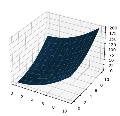
%%timeit
z_interp = interp(np.column_stack((x_new.ravel(), y_new.ravel()))).reshape(x_new.shape)
44.5 μs ± 824 ns per loop (mean ± std. dev. of 7 runs, 10,000 loops each)
Here we introduce MultivariateInterp, which brings additional features and speed improvements. The key feature of MultivariateInterp is its backend parameter, which can be set to scipy, numba, or cupy, among others. This allows the user to specify the backend device for the interpolation. Using MultivariateInterp mirrors the use of RegularGridInterpolator very closely.
mult_interp = MultivariateInterp(z_mat, [x_grid, y_grid])
z_mult_interp = mult_interp(x_new, y_new)

# Plot
fig, ax = plt.subplots(subplot_kw={"projection": "3d"})
ax.plot_surface(x_new, y_new, z_mult_interp)
plt.show()
%%timeit
z_mult_interp = mult_interp(x_new, y_new)18.1 μs ± 377 ns per loop (mean ± std. dev. of 7 runs, 100,000 loops each)
As we see above, MultivariateInterp is faster than RegularGridInterpolator, even with the default backend="scipy". Moreover, the speed of MultivariateInterp is highly dependent on the number of points in the grid and the backend device. For example, for a large number of points, MultivariateInterp with backend='numba' can be shown to be significantly faster than RegularGridInterpolator.
gpu_interp = MultivariateInterp(z_mat, [x_grid, y_grid], backend="cupy")
z_gpu_interp = gpu_interp(x_new, y_new).get()  # Get the result from GPU
%%timeit
z_gpu_interp = gpu_interp(x_new, y_new).get() # Get the result from GPU766 μs ± 130 μs per loop (mean ± std. dev. of 7 runs, 1,000 loops each)
We can test the results of MultivariateInterp against RegularGridInterpolator, and we see that the results are almost identical.
np.allclose(z_interp - z_gpu_interp, z_mult_interp - z_gpu_interp)TrueTo experiment with MultivariateInterp and evaluate the conditions which make it faster than RegularGridInterpolator, we can create a grid of data points and interpolation points and then time the interpolation on different backends.
n = 35
grid_max = 300
grid = np.linspace(10, grid_max, n, dtype=int)
fast = np.empty((n, n))
scipy = np.empty_like(fast)
parallel = np.empty_like(fast)
gpu = np.empty_like(fast)
We will use the following function to time the execution of the interpolation.
def timeit(interp, x, y, min_time=1e-6):
    if isinstance(interp, RegularGridInterpolator):
        start = time()
        points = np.column_stack((x.ravel(), y.ravel()))
        interp(points).reshape(x.shape)
    else:
        interp.compile()
        start = time()
        interp(x, y)

    elapsed_time = time() - start
    return max(elapsed_time, min_time)
For different number of data points and approximation points, we can time the interpolation on different backends and use the results of RegularGridInterpolator to normalize the results. This will give us a direct comparison of the speed of MultivariateInterp and RegularGridInterpolator.
for i, j in product(range(n), repeat=2):
    data_grid = np.linspace(0, 10, grid[i])
    x_cross, y_cross = np.meshgrid(data_grid, data_grid, indexing="ij")
    z_cross = squared_coords(x_cross, y_cross)

    approx_grid = np.linspace(0, 10, grid[j])
    x_approx, y_approx = np.meshgrid(approx_grid, approx_grid, indexing="ij")

    fast_interp = RegularGridInterpolator([data_grid, data_grid], z_cross)
    time_norm = timeit(fast_interp, x_approx, y_approx)
    fast[i, j] = time_norm

    scipy_interp = MultivariateInterp(z_cross, [data_grid, data_grid], backend="scipy")
    scipy[i, j] = timeit(scipy_interp, x_approx, y_approx) / time_norm

    par_interp = MultivariateInterp(z_cross, [data_grid, data_grid], backend="numba")
    parallel[i, j] = timeit(par_interp, x_approx, y_approx) / time_norm

    gpu_interp = MultivariateInterp(z_cross, [data_grid, data_grid], backend="cupy")
    gpu[i, j] = timeit(gpu_interp, x_approx, y_approx) / time_norm
fig, ax = plt.subplots(1, 3, sharey=True)
ax[0].imshow(
scipy,
cmap="RdBu",
origin="lower",
norm=colors.SymLogNorm(1, vmin=0, vmax=10),
interpolation="bicubic",
extent=[0, grid_max, 0, grid_max],
)
ax[0].set_title("scipy")
ax[1].imshow(
parallel,
cmap="RdBu",
origin="lower",
norm=colors.SymLogNorm(1, vmin=0, vmax=10),
interpolation="bicubic",
extent=[0, grid_max, 0, grid_max],
)
ax[1].set_title("numba")
cbar = ax[2].imshow(
gpu,
cmap="RdBu",
origin="lower",
norm=colors.SymLogNorm(1, vmin=0, vmax=10),
interpolation="bicubic",
extent=[0, grid_max, 0, grid_max],
)
ax[2].set_title("cupy")
cbar = fig.colorbar(
cbar,
ax=ax,
label="Relative Speed (faster - slower)",
location="bottom",
)
cbar.set_ticks([0, 0.1, 0.5, 1, 2, 5, 10])
cbar.set_ticklabels(["0", "0.1", "0.5", "1", "2", "5", "10"])
ax[0].set_ylabel("Data grid size (squared)")
ax[1].set_xlabel("Approximation grid size (squared)")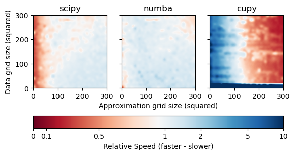
As we can see from the results, MultivariateInterp is faster than RegularGridInterpolator depending on the number of points and the backend device. A value of 1 represents the same speed as RegularGridInterpolator, while a value less than 1 is faster (in red) and a value greater than 1 is slower (in blue).
For backend="scipy", MultivariateInterp is (much) slower when the number of approximation points that need to be interpolated is very small, as seen by the deep blue areas. When the number of approximation points is moderate to large, however, MultivariateInterp is about as fast as RegularGridInterpolator.
For backend="numba", MultivariateInterp is slightly faster when the number of data points with known function value are greater than the number of approximation points that need to be interpolated. However, backend='parallel' still suffers from the high overhead when the number of approximation points is small.
For backend="cupy", MultivariateInterp is much slower when the number of data points with known function value are small. This is because of the overhead of copying the data to the GPU. However, backend='numba' is significantly faster for any other case when the number of approximation points is large regardless of the number of data points.
Copyright © 2024 Lujan. This is an open-access article distributed under the terms of the Creative Commons Attribution 4.0 International license, which enables reusers to distribute, remix, adapt, and build upon the material in any medium or format, so long as attribution is given to the creator.
- GPU
- Graphics Processing Unit