from __future__ import annotations

import matplotlib.pyplot as plt
import numpy as np
from multinterp.unstructured import UnstructuredInterp
Suppose we have a collection of values for an unknown function along with their respective coordinate points. For illustration, assume the values come from the following function:
def function_1(u, v):
    return u * np.cos(u * v) + v * np.sin(u * v)
The points are randomly scattered within a square and therefore have no regular structure.
rng = np.random.default_rng(0)
rand_x, rand_y = rng.random((2, 1000)) * 3
values = function_1(rand_x, rand_y)
Now suppose we would like to interpolate this function on a rectilinear grid, which is known as “regridding”.
grid_x, grid_y = np.meshgrid(
    np.linspace(0, 3, 100),
    np.linspace(0, 3, 100),
    indexing="ij",
)
To do this, we use multinterp’s UnstructuredInterp class. The class takes the following arguments:
values: an ND-array of values for the function at the pointsgrids: a list of ND-arrays of coordinates for the pointsmethod: the interpolation method to use, with options “nearest”, “linear”, “cubic” (for 2D only), and “rbf”. The default is'linear'.
The UnstructuredInterp class is an object oriented wrapper around scipy.interpolate’s functions for multivariate interpolation on unstructured data, which are NearestNDInterpolator, LinearNDInterpolator, CloughTocher2DInterpolator, and RBFInterpolator. The advantage of using multinterp’s UnstructuredInterp class is that it provides a consistent interface for all of these methods, making it easier to switch between them and other interpolators in the multinterp package.
nearest_interp = UnstructuredInterp(values, (rand_x, rand_y), method="nearest")
linear_interp = UnstructuredInterp(values, (rand_x, rand_y), method="linear")
cubic_interp = UnstructuredInterp(values, (rand_x, rand_y), method="cubic")
rbf_interp = UnstructuredInterp(values, (rand_x, rand_y), method="rbf")
Once we create the interpolator objects, we can use them using the __call__ method which takes as many arguments as there are dimensions.
nearest_grid = nearest_interp(grid_x, grid_y)
linear_grid = linear_interp(grid_x, grid_y)
cubic_grid = cubic_interp(grid_x, grid_y)
rbf_grid = rbf_interp(grid_x, grid_y)
Now we can compare the results of the interpolation with the original function. Below we plot the original function and the sample points that are known.
true_grid = function_1(grid_x, grid_y)
plt.imshow(true_grid.T, extent=(0, 3, 0, 3), origin="lower")
plt.plot(rand_x, rand_y, "ok", ms=2, label="input points")
plt.title("Original")
plt.legend(loc="lower right")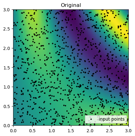
Then, we can look at the result for each method of interpolation and compare it to the original function.
fig, axs = plt.subplots(2, 2, figsize=(6, 6))
titles = ["Nearest", "Linear", "Cubic", "Radial basis function"]
grids = [nearest_grid, linear_grid, cubic_grid, rbf_grid]

for ax, title, grid in zip(axs.flat, titles, grids):
    im = ax.imshow(grid.T, extent=(0, 3, 0, 3), origin="lower")
    ax.set_title(title)

plt.tight_layout()
plt.show()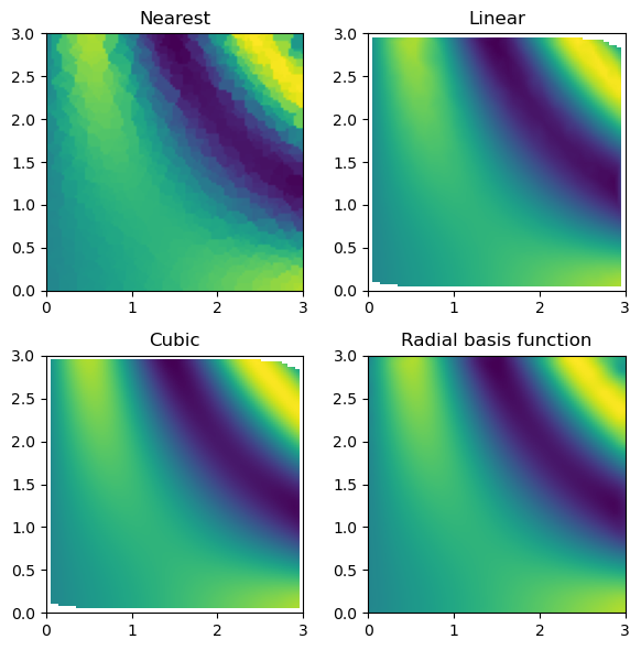
Finally, multinterp also provides a set of interpolators organized around the concept of regression. As a demonstration, below we use a RegressionUnstructuredInterp interpolator which uses a Gaussian Process regression model from scikit-learn (Pedregosa et al. (2011)) to interpolate the function defined on the unstructured grid. The RegressionUnstructuredInterp class takes the same arguments as the UnstructuredInterp class, but it additionally requires the user to specify the regression model to use.
from multinterp import RegressionUnstructuredInterp

gaussian_interp = RegressionUnstructuredInterp(
    values,
    (rand_x, rand_y),
    model="gaussian-process",
    std=True,
)

gaussian_grid = gaussian_interp(grid_x, grid_y)

fig, axs = plt.subplots(1, 2, figsize=(6, 6))
titles = ["Original", "Gaussian Process"]
grids = [true_grid, gaussian_grid]

for ax, title, grid in zip(axs.flat, titles, grids):
    im = ax.imshow(grid.T, extent=(0, 3, 0, 3), origin="lower")
    ax.set_title(title)

plt.tight_layout()
plt.show()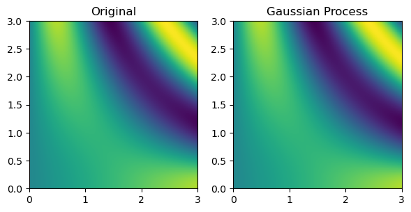
Copyright © 2024 Lujan. This is an open-access article distributed under the terms of the Creative Commons Attribution 4.0 International license, which enables reusers to distribute, remix, adapt, and build upon the material in any medium or format, so long as attribution is given to the creator.
- Pedregosa, F., Varoquaux, G., Gramfort, A., Michel, V., Thirion, B., Grisel, O., Blondel, M., Louppe, G., Prettenhofer, P., Weiss, R., Weiss, R. J., Vanderplas, J., Passos, A., Cournapeau, D., Brucher, M., Perrot, M., & Duchesnay, E. (2011). Scikit-learn: Machine Learning in Python. Journal of Machine Learning Research: JMLR, abs/1201.0490, 2825–2830.