
Numba v2: Towards a SuperOptimizing Python Compiler
Abstract
This paper presents early work on Numba v2, a general-purpose compiler for Python that integrates equality saturation (EqSat) as a foundation for program analysis and transformation. Whilst inspired in part by the needs of AI/ML workloads, and also supporting tensor optimizations, Numba v2 is not a tensor-oriented compiler. Instead, it provides a flexible framework where user-defined mathematical and domain-specific rewrites participate in the compilation process as a complement to the compilation supported by Numba today. This paper outlines the design of Numba v2’s EqSat-based compiler and its potential to serve as an extensible, superoptimizing compiler for a broad range of numerical and scientific Python applications.
1Introduction
The Numba team is developing a new version of the Numba compiler (Numba v2)[1] to meet the evolving computational demands of the modern workloads, including, but not limited to, those in AI/ML. Whilst these domains have popularized high-level optimization techniques based on tensor-oriented programming, Numba v2 is not a specialized tensor compiler; instead, it is a general-purpose compiler that supports tensors. It integrates equality saturation (EqSat) as a core mechanism for program analysis and transformation. The use of EqSat allows the compiler to blend user-defined mathematical rewriting and other domain specific rewriting into the transformation pipeline for compiling numerically oriented Python code with loop and branch constructs. Although Numba v2 is still under active development, this paper presents its new EqSat-based compilation strategy as a foundation for an extensible superoptimizing[2] compiler.
1.1The importance of mathematical rewrites
AI/ML has popularized tensor-oriented programming. In contrast to array-oriented programming, where an array is a data-structure without mathematical meaning, tensor-orientated programming has an associated mathematical nature. This move to such higher level abstractions allows the compiler to manage low-level details such as buffer reuse, DMA transfers[3] to accelerators, and even asynchronous transfers in distributed systems. It also enables the compiler to do analysis and perform optimizations in terms of the mathematical properties of tensors.
One of the challenges with the currently hugely popular large-language models (LLMs) is that Transformers are computationally expensive. Dao, 2023 manually optimized the Attention layer in Transformers to improve performance, building on FlashAttention’s Dao et al., 2022 fusing of the softmax operation into the matrix-multiply operation. A reviewer of the paper asked why compilers couldn’t perform the necessary fusion, to which the author answered:
Compilers can generally perform fusion. However, optimizations that require mathematical rewriting of the same expression (while maintaining numerical stability) are generally harder for compilers.
—- Dao (2023) answering why compiler cannot create FlashAttention-2
The gap between what practitioners need and what compilers can provide is fulfilled by mathematical rewrites, expressed strategically using domain knowledge to allow for more aggressive optimization. In this paper, the use of EqSat is proposed to address this issue. EqSat allows mathematical rewrites and other code transformations to be expressed in declarative logical rules. The compiler can then explore all program variants derived from these rules, hence saturation. Finally, the optimal program variant is obtained via a cost-based extraction. This approach leads to a superoptimizing compiler.
1.2Phase ordering problems in Numba v1
Numba v1 suffers from the phase-ordering problem—a well-known challenge in compiler design where the order of compiler passes can significantly impact the result. EqSat offers a principled solution by exploring all rewrite possibilities simultaneously without a specific order.
Numba v1 works by translating the Python bytecode for a function into an intermediate representation (IR) called Numba IR. Type inference is run on this to statically type the variables, it is then lowered to LLVM IR, which is then JIT compiled using the LLVM compiler infrastructure. For details see Lam et al. (2015).
The Python bytecode is an IR executed by the Python virtual machine, it is necessarily low level, so much so that the majority of the semantics expressed in source code, for example array expressions, are entirely lost once encoded into bytecode and must be rediscovered later in the compiler pipeline. Numba’s IR is a near direct translation of Python bytecode and therefore also lacks high-level semantic information from the original source. As a result, recovering the programmer’s intent requires significant analysis of the Numba IR, including control-flow reconstruction and type inference. This problem manifests itself acutely when, for example, trying to identify regions of code which are suitable for parallel execution or when trying to prove amenability for array expression fusion.
Following bytecode to Numba IR translation, the next step in compilation is type inference. This is the process of determining the type of all the variables in use. It is quite hard to do this using fixed-point iterative algorithms, particularly when protocol based code is being compiled (code using “dunder” methods). This is because types have to be propagated through the system, and then branches pruned and inlining performed based on the arrival of concrete type information, which then in turn may expose further areas of code that subsequently need further rounds of type propagation, branch pruning and inlining. The interdependence creates a cascading effect that is difficult to manage in a naive pass-based fixed-point iteration scheme. Essentially this is a compiler pass phase ordering problem with no guarantee that the type propagation will stabilize. A further side effect of this sort of problem, and incremental type inference in general, is that back-tracking invalid paths is computationally wasteful and is hard to debug. It also makes it hard to e.g. pass an untyped list into a function and to permit compilation to continue with the view that the type may be resolved eventually.
1.3A motivating case
To demonstrate some of these issues in relation to compiler flexibility and optimisation, a motivating example of the associativity of matrix multiplication can be used. In this example, six matrices are being multiplied together:
Using NumPy syntax, it looks like this:
def six_matrix_multiply(A1, A2, A3, A4, A5, A6):
return A1 @ A2 @ A3 @ A4 @ A5 @ A6
From Numba v1’s perspective, it will analyse the bytecode and create some Numba
IR which will naively store the result from each operation in the chain into a
temporary variable for use in the next operation. Type inference will then run
and work out that each @ is actually a numpy.dot operation and will resolve
that as a function that will take two array inputs and return an array output.
Numba will then lower this typed Numba IR to a chain of (wrapped) BLAS GEMM
calls, with Numba’s built-in runtime providing the memory buffers for the array
temporaries.
Whilst Numba v1 did resolve the types correctly within its type system, because its type system is hard to extend, it cannot be made to go further and do the necessary shape inference needed to be able to optimise the sequence of matrix multiplications. Arguably Numba v1 could have a custom optimisation pass added to its pipeline that operates on the low level Numba IR and rewrites it to try and reuse memory buffers associated with temporaries and perhaps looks at the matrix memory ordering to try and improve cache utilization. However, this would be a very custom compiler pass, tuned to this one situation, and almost certainly quite hard to write.
Now imagine applying a Numba v2 that doesn’t have the limitations of v1 to the same problem. First a higher-level IR is emitted than that comes from the bytecode. Subsequently, both type and shape inference are performed to identify the exact shapes of all the arrays in the computation. This now leads to an interesting problem, in that the shapes and operations are all known, but optimising this is incredibly hard in part because the problem space is so large. In fact, the number of possible grouping under the associativity rule is the Catalan number .
Consider that matrix multiplication is a well defined problem and that the approximate floating point cost of for multiplying matrices is . Furthermore, the associativity rule for multiplication is well known and easily expressed. There is now a problem space forming where the operations are known, the types and shapes of the operands are known, rules of associativity could be applied, and a cost is available for all operations. An optimal solution exists, but as noted before, the space is large. To solve this problem a new technique is employed, that of superoptimization via equality saturation. This technique uses a set of rewrite rules and effectively builds all possible programs simultaneously. It then assigns costs to each expression and then uses a cost model to extract the optimal solution.
2Developing an Equality Saturation based solution
The ideas behind equality saturation lie in the e-graph data structure, which in turn originates from automatic theorem provers Nelson, 1980 and SAT solvers Moura & Bjørner, 2008, where it was used to efficiently represent congruence closure. More recently, this theory has been adapted into the powerful equality saturation (EqSat) technique, which has enabled term-rewriting-based compiler optimizations (Willsey et al. (2020), Zhang et al. (2023)).
Traditional term rewriting systems rely on fixed rule application schedules, discarding the original term after each rewrite. As a result, their effectiveness depends heavily on carefully designed transformation pass orderings, which are often brittle and unable to guarantee optimal results across all cases. Some systems mitigate this by using backtracking Jia et al., 2019, where previous terms are restorable, but this approach is computationally expensive, as all alternatives must be evaluated sequentially. EqSat addresses this by applying all rewrite rules simultaneously and retaining all resulting variants. It efficiently stores these alternatives by grouping semantically equivalent terms into equivalence classes (e-classes), with each e-class containing multiple e-nodes each representing equivalent program terms. This structure enables substantial reductions in both search time and memory usage, allowing the compiler to explore the full space of program variants without requiring explicit rule application schedules. Consequently, EqSat eliminates phase-ordering problems and promotes a more composable and extensible compiler architecture.
EqSat and the ability to easily employ rewriting rules exposes a realm of optimisation capabilities that were not previously available. For example, if it is known that the application domain is deep-learning, then floating point error tolerance is likely quite high and various rewrite rules to exploit this situation could be applied. First, it is possible to use lower-precision data types such as 8-bit floats or even 4-bit floats. If the application needs to be deployed on an industrial scale that serves thousands of requests per second, or at the edge running on power-limited mobile phone processors, the power usage becomes an important factor as well. Use of integer addition to approximate the floating point multiplication for lower power scenarios is another option. The computation could be done as an approximation, maybe as a low-rank approximation via SVD compression. All of these possibilities are encodable as rewrite rules and become part of the possible solution space within the equality saturation based optimiser. Extracting the optimal solution just becomes a question of defining a cost model that is appropriate to the domain e.g. performance, power cost, code size, hardware.
3Compiler Design
3.1Architecture Overview
Numba v2 architecture follows the conventional structure of many compilers; a frontend for canonicalising and translating an input language into an intermediate form, a middle end for performing optimisations and a backend for translating the intermediate form into an executable. The following sections explain the process in more detail and should be read in conjunction with the following diagram.

Figure 1:Compiler architecture
A key architectural distinction between Numba v1 and v2 lies in their treatment of middle-end optimization. Numba v1 has a minimal middle-end that handles type resolution and basic IR transformations before lowering to LLVM IR. This design places the optimization burden on LLVM’s backend passes. This architectural shift enables optimizations that are fundamentally inaccessible to v1’s pipeline, as demonstrated by the 19× speedup achieved in Section 4.2 through purely algebraic reorganization.
3.2Converting imperative Python to functional form
As noted above, to use egglog effectively, the Python AST is first translated into an S-expression form that supports term rewriting. A direct encoding of the AST into S-expression form is insufficient, as it captures only the syntactic structure of the program. The goal, however, is to perform term rewriting based on semantic equivalence and so the syntactic form is translated into a semantic representation. An additional challenge is that Python is an imperative language with implicit state mutations. To accommodate the necessary semantics, the AST is converted into a regionalized value-state dependence graph (RVSDG).
RVSDG is a data-oriented program representation that can simplify compiler analysis and transformation. Unlike the common SSA-CFG IRs[4], RVSDG does not explicitly encode the control-flow graph (CFG). Prior studies (Reissmann et al. (2019), Weise et al. (1994), Lawrence (2007)) have shown that RVSDG enables faster and simpler implementations of classical compiler passes. This reflects a broader trend towards data-dependency based compilation, even for imperative languages, as evidenced by frameworks like MLIR Lattner et al., 2021.
In RVSDG, programs are represented in terms of dataflow graphs, where edges indicate value and state dependencies, and nodes denote computation. Structured control flow is modelled using regions that encapsulate other nodes and edges, resembling block diagrams in digital circuit design. Within this structure, parallelization opportunities appear as independent groups of nodes.
There are three types of structured control flow regions: linear dependency, switches for optional paths, and tail loops. The resulting graph is an acyclic graph with nested regions, making it amenable to hierarchical analysis. Every node, including control-flow regions, in an RVSDG is an operation with incoming and outgoing “ports” for values and states.
Following the algorithms outlined in Bahmann et al. (2015), the Python AST is
first converted into a structurized control-flow graph[5], each
imperative Python expression is then converted into an RVSDG-conforming
S-expression by explicitly passing an io state through each operation. Any
operation with side-effects receives and returns an io state. Initially, all
Python operations are conservatively assumed to have side-effects. This
assumption can later be relaxed through analysis such as type-inference, which
is done using the same EqSat rule mechanism as other code transformations.
This approach differs from prior work on Program Expression Graphs (PEGs) Stepp, 2011, which handle effects through a single global state token. RVSDG simplifies effect handling by using explicit state edges within hierarchical regions that naturally enforce sequential ordering through structured control flow representation.
3.3Controlflow handling and semantic raising
Encoding Python into RVSDG is conceptually similar to translating Python into a
pure functional language. In this representation, all operations appear pure
because state is passed as a first-class value. An effect-free operation is
simply one that doesn’t modify the io state. Many traditional compiler passes
are simplified in RVSDG because of the uniform treatment of states and values.
Since there is no control-flow graph, as the program is viewed in a
data-oriented perspective, control-flow constructs, such as conditionals and
loops, are treated like any other operations. This eliminates the need for
specialized logic to handle control-flow and reduces the complexity of compiler
passes.
Practically, the compiler uses an S-Expression based IR as an RVSDG based functional encoding suitable for translating into the egglog Python library bindings. At this point, the Python program is in a form in which rewrite rules can be written and subsequently applied through EqSat.
E-graph rewrite rules are akin to logic programming. They operate declaratively without specifying application strategy and are therefore inherently composable. The rewrite system uses pattern matching to identify transformable program structures and conditional guards to ensure transformation validity. Each rule specifies a source pattern to match against the e-graph and a target pattern representing the equivalent transformation, with optional conditions that must hold for the rewrite to apply. For example, the constant folding ruleset below demonstrates how conditional branches with constant predicates can be simplified:
@ruleset
def ruleset_const_fold_if_else(a: Term, b: Term, c: Term, operands: TermList):
    yield rewrite(
        # Define the if-else pattern to match
        Term.IfElse(cond=a, then=b, orelse=c, operands=operands),
        subsume=True,  # subsume to disable extracting the original term
    ).to(
        # Define the target expression
        # This applies region `b` (then) using the `operands`.
        Term.Apply(b, operands),
        # Given that the condition is constant True
        IsConstantTrue(a),
    )
    yield rewrite(
        # Define the if-else pattern to match
        Term.IfElse(cond=a, then=b, orelse=c, operands=operands),
        subsume=True,  # subsume to disable extracting the original term
    ).to(
        # Define the target expression.
        # This applies region `c` (orelse) using the `operands`.
        Term.Apply(c, operands),
        # Given that the condition is constant False
        IsConstantFalse(a),
    )
The Term.IfElse node represents a conditional expression in RVSDG.
Simplifying it is straightforward when the condition is a constant. A pattern
matching rewrite rule replaces the entire if-else construct with the
corresponding selected branch. The logic is intuitive and compact when
expressed in the declarative rule system of egglog. The simplicity of this
transformation highlights the benefits of treating control flow as just another
term in the rewrite system.

Figure 2:This illustrates the process of applying the if-else simplification rewrite rule on the e-graph. Each blue box represents an e-node. The dotted box represents e-classes—blue-boxes inside are equivalent to each other. The left diagram is the initial state. The center diagram shows the condition (Cond) is recognized as a constant True. The right diagram shows the establishing of equivalence between the IfElse term and the Then term.
Loops presents a greater challenge as RVSDG supports only tail-controlled loops, while Python uses constructs like while-loop and for-loop that do not naturally fit this mode. To bridge this gap to allow for more intuitive reasoning in EqSat, semantic raising is employed to recover the high-level Python loop constructs by matching their low-level RVSDG patterns. This allows full recovery of Python loop semantics from raw RVSDG form, enabling use of more intuitive rewrite rules.
As an example, RVSDG restructurization converts a for-loop into the following CFG structure.
condition = compute_init_loop_condition()
do {
    if condition {
        condition, vals = loop_body(*vals)
    }
} while condition
Through semantic raising, the loop structure above can be “raised into a more abstract representation:
Py_ForLoop(iterator, operands) { loop_body }To recognize the pattern as a for ... in range loop, which is common in
numerical code, further semantic raising can be employed. This high-level
representation enables a more direct mapping to MLIR’s affine dialect.
3.4Limitations of EqSat
One known challenge of EqSat is that saturation can create very large e-graphs that exceed the memory limits of a given machine. In the case of Numba v2, this issue has not arisen as the project is still in its early stages. However, prior work provides insight into techniques for managing e-graph growth.
Thomas & Bornholt (2024) reintroduce phases into the rewriting process to control the e-graph expansion. They break rewriting into three phases:
Expansion phase: explores alternative unoptimized program variants; e.g. applying math identities.
Compilation phase: converts unoptimized terms to optimized ones.
Optimization phase: searches for better representation among optimized terms.
To prevent unbounded graph growth, they also employ cost-based pruning, using an abstract cost model to select the best intermediate program after expansion and compilation phase. Saturation in these phases is bounded by a time limit and only once improvements plateau, according to the abstract cost model, the optimization phase is applied.
Koehler et al. (2021) offer a different approach. Instead of optimizing directly over full program representations, they use program sketches—compressed abstractions of the full program—to guide optimization. This helps reduce e-graph size and keeps optimization tractable.
These concerns are particularly relevant for compilers that target low-level
representations, such as ISA or machine code, where program representations can
be enormous In contrast, Numba v2 applies EqSat at a much higher level.
Low-level optimizations are delegated to MLIR. High-level program
representations tend to be significantly smaller, and MLIR supports expressive
dialects that further reduce complexity. For example, recognizing and
translating a for … in range loop into MLIR’s affine dialect can eliminate
many low-level details and shrink the overall program graph.
3.5Cost-based extraction
The cost-based extraction in Numba v2 is built around three guiding principles:
Intuitive: it should be intuitive for users to express cost equations naturally for each operation in the cost model.
Stability. Cost-computation must be stable such that the computed cost of any subprogram remains consistent across different compilations so as to ensure reproducibility.
Fast. Practicality and performance are prioritized even at the expense of finding the absolute optimal solution, especially given the scale of real-world programs.
In the generalized case, costs are modelled as vectors of floats, allowing for future experimentation with multi-objective evaluation. Finding the exact minimal cost extraction from an e-graph is NP-hard Sun et al., 2024. An iterative relaxation algorithm is used to manage this complexity and to efficiently handle cycles in the e-graph, so as to permit convergence to a near-optimal solution.
3.6Iterative relaxation algorithm
The extraction algorithm is inspired by the Bellman-Ford algorithm Bellman, 1958, combining dynamic programming with iterative refinement. It decomposes the extraction problem into subproblems, computing an initial best-effort solution that is progressively improved upon as more information becomes available in subsequent iterations. Unlike Dijkstra-based approaches commonly used in other e-graph systems [6], Bellman-Ford permits negative costs, though these are not currently required in the Numba v2 test cases. The iterative nature also offers a practical advantage by allowing early termination based on a time budget.
The algorithm has the following steps:
Dependency graph construction: Starting from the root e-class (the function definition term), the algorithm traces its member e-nodes. Each e-node references child e-classes, forming a dependency graph. In this graph, e-classes point to e-nodes, and e-nodes point to their child e-classes.
Cost function retrieval: For each e-node, the algorithm retrieves the associated cost function used to compute its contribution to the total cost.
Identify constant values: Constant values that participate in cost calculations are identified, such as the shape of a tensor in a matrix multiplication operation.
Compute the BFS layers: Since the dependency graph may contain cycles, a true topological sort is not possible. Instead, breadth-first search (BFS) layers are used to approximate topological ordering.
Iterate until convergence: The cost is computed bottom-up for each e-node by using the cost of its child e-classes in the e-node’s cost function. If the child e-class has not yet been evaluated, its cost is temporarily treated as infinite. Each e-class aggregates the costs of its member e-nodes and selects the best. The algorithm continues until convergence. The criteria for convergence are:
The number of finite-cost e-nodes remains unchanged.
The maximum cost change falls below a predefined threshold
By construction, e-nodes form a directed acyclic graph (DAG) since they
represent RVSDG terms and only reference the operands (child nodes). However,
cycles can arise through e-node merging during rewriting. For example, the
identity pow(x, 1) = x causes both expressions to reside in the same e-class,
creating a cyclic self reference. These cycles are not problematic and they are
resolved early in the relaxation process. Once a lower cost is found for a
node, it is immediately selected as the currently optimal choice, effectively
breaking the cycle.
3.7Dual cost model
Accurate cost-based extraction of the e-graph requires careful handling of differing cost aggregation requirements for expression DAGs and control-flow DAGs.
In the e-graph, expressions are represented as DAGs where nodes may be shared
in other expressions. Since the cost is computed locally for each operation
without full visibility to the entire graph structure due to the bottom up
traversal, common subexpression can be counted more than once in an expression
tree. For example, x * x * x can redundantly count the cost of x multiple
times (See Figure 3) , making it appear more expensive than pow(x, 3).
To avoid this, node-based cost accounting is performed to properly recognize
shared expression nodes.
Control-flow operations such as loops require a different treatment. A loop’s
cost should reflect its trip count multiplied by the cost of its body. Unlike
shared subexpressions in expression DAGs, the cost of the loop-body is not
discounted, even if it appears in other parts of the program. This calls for
edge-based cost accounting. For example, in Figure 4, the cost of Body
should contribute to the cost of both Loop1 and Loop2.
A dual cost model is adopted to resolve the conflicting situation:
Local cost computation. Each e-node defines a cost equation that receives the costs of its child nodes (operands). For example, a loop operation might compute its cost as the cost of the loop body multiplied by the trip out. For simple operations like scalar addition, the cost is simply a constant. These local cost functions can be user-defined and customizable.
Child-dependent cost computation. To handle shared subexpression nodes, an external cost that aggregates the costs of a node’s children without duplication is computed. This requires tracking the optimal e-node for each e-class along with its total cost (local + external). During extraction, the full set of contributing e-nodes is computed to ensure that each e-node is only counted once. This approach is similar to the FasterGreedyDagExtractor.

Figure 3:This illustrates the expression x * x * x. The cost of node #1 is the local_cost#1 + local_cost#2 + local_cost#3.

Figure 4:This illustrates a function with two loops, for which the loop-bodies are equivalent in the e-graph. The function (#0) has a cost that is the sum of all local costs of its unique children. In Loop1 (#1) and Loop2 (#2) the cost of the Body is contributing to their local costs, respectively.
3.8Evaluating Scalability
A scalability analysis was conducted by scaling the matrix multiplication associativity example from Section 4.2 to an increasing number of operations. Here, represents the number of matrices, and corresponds to the number of matrix multiplications. This subjects the compiler to a pathological scenario due to the combinatorial explosion caused by the associativity rule. Figure 5 shows that the e-graph exhibits polynomial scaling behavior. The number of e-classes shows sub-quadratic growth () while the number of e-nodes exhibits sub-cubic growth (). This growth rate is substantially lower than the theoretical exponential rate because e-graphs inherently perform structural matching that compresses the representation.
Both saturation and extraction phases exhibit sub-quadratic scaling () w.r.t. number of e-classses. In practice, such pathological cases of long chains of associative operations are uncommon, and since associativity rules serve only optimization purposes, compilation time can be capped as needed. The sub-quadratic growth ensures EqSat remains tractable for realistic numerical programs.
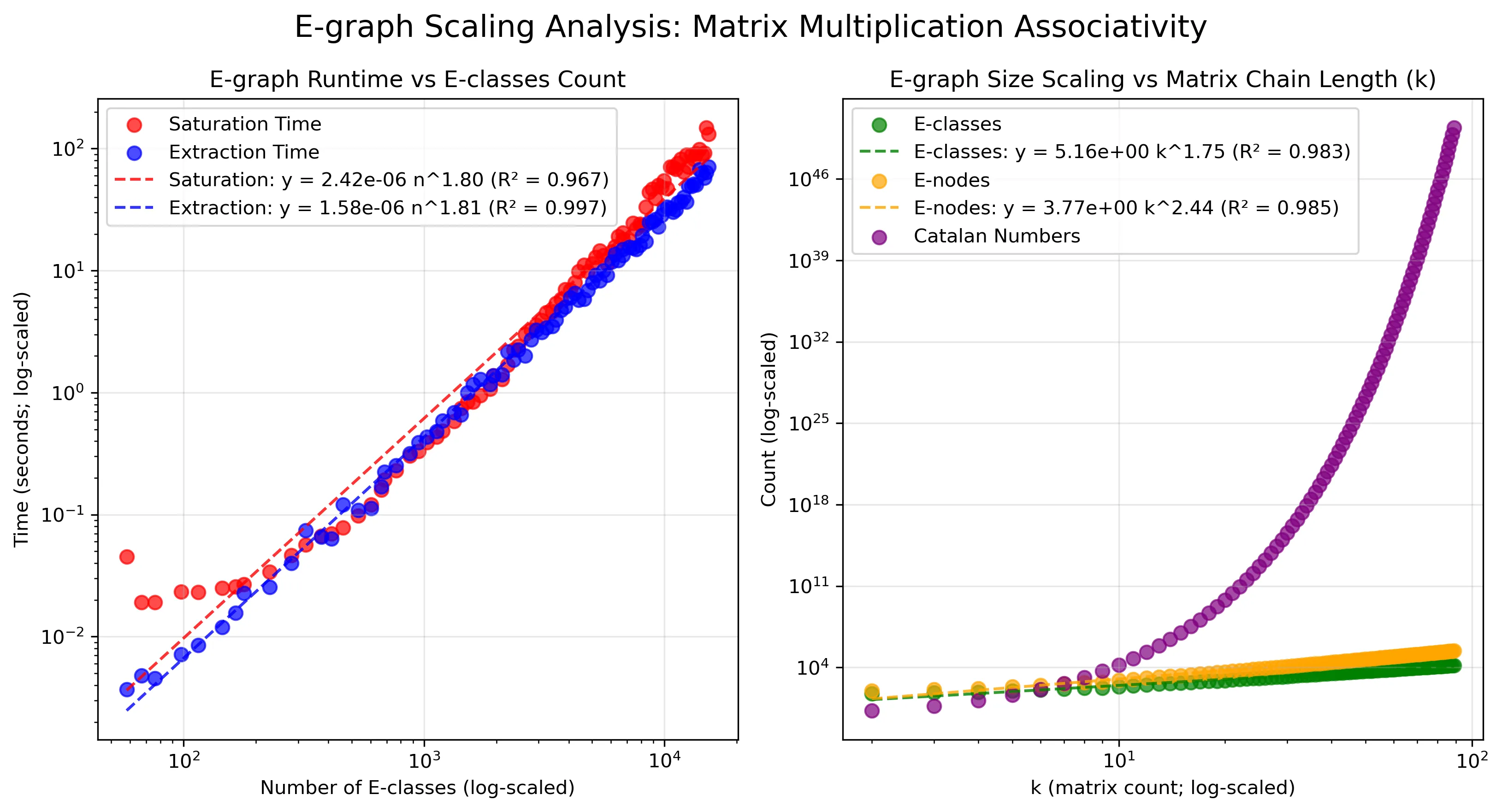
Figure 5:(a) Left: saturation and extraction time scaling w.r.t. e-graph size. (b) Right: e-graph size scaling w.r.t. matrix-multiplication chain length.
3.9Further considerations
This work represents an early stage in the substantial development work of Numba v2. While initial results are promising, future efforts will need to scale to more realistic examples, focus on refining the techniques, and conduct deeper analysis.
Larger and whole-program examples
To better evaluate the effectiveness and scalability of this technique, testing on more complex and realistic programs is needed. As part of this effort, the next goal is to compile a NumPy-based implementation of a small LLaMa based LLM Park, 2024.
Extending to multi-dimensional cost models. The cost-based extraction algorithm is designed to support n-dimensional cost vectors, enabling multi-objective optimization (e.g. runtime, memory usage, floating-point accuracy, power). So far, the examples have primarily used 1-dimensional cost, but future work will explore richer cost models.
4Case Studies
4.1GELU Approximation
Traditional compilers have limited ability to relax floating-point precision. Many expose a fast-math flag that enables basic operation reassociation or using fused multiply-add instruction, but they typically lack more advanced capabilities such as replacing transcendental functions with cheaper approximations.
In domains like deep learning, it’s often possible to speed up programs by reducing the precision of specific functions. Activation functions are a good candidate for this kind of optimization.
As a concrete example, GELU (Gaussian Error Linear Unit), which is a common in some transformer architectures Hendrycks & Gimpel, 2016, is used.
GELU equation:
The Python implementation:
def gelu_tanh_forward(x):
    dt = np.float32
    erf = np.tanh(np.sqrt(dt(2) / dt(np.pi)) * (x + dt(0.044715) * x**3))
    return dt(0.5) * x * (dt(1) + erf)
Pade44 approximation is used to simplify the tanh(x) function:
In egglog, the rewrite rule for it is expressed as below:
rewrite(Npy_tanh_float32(x)).to(
    div(
        add(mul(flt(10), pow(x, liti64(3))), mul(flt(105), x)),
        add(
            add(pow(x, liti64(4)), mul(flt(45), pow(x, liti64(2)))),
            flt(105),
        ),
    )
)
The corresponding formal inference rule representation of the rewrite rule is:
This can combine with a simplification of the pow(x, constant) term with the identity:
As egglog rules:
rewrite(pow(x, lit64(ival))).to(
    mul(x, pow(x, lit64(ival - 1))),
    ival >= 1,
)
rewrite(pow(x, lit64(i64(0))), subsume=True).to(
    Npy_float32(Term.LiteralF64(float(1))),
)
The corresponding formal inference rule representation of the rewrite rule is:
Egglog saturates these rules, so there is no need to specify an ordering or how
many times to apply them. For example, pow() calls are automatically expanded
into multiplications after the applying the pade44 approximation for tanh().
As a result, user programs can be optimized without requiring direct modifications. Each rewrite rule is also reusable across different programs. Performance evaluation demonstrates 9× speedup for superoptimized code using MLIR code generation compared to Numba v1, which fails to achieve speedup over vanilla Python due to computation dominated by transcendental functions.
Two ways are envisioned for users to take advantage of this kind of program rewriting.
The first is by manual selection from a catalog of rewrite rules. Users will need domain knowledge to choose rules that are appropriate for their use case.
The second is to use a cost model to guide the selection of approximation functions. The cost model can be extended to account not only for runtime performance but also for floating-point accuracy.
4.2Associativity Rule of Matrix Multiply
In the introduction, there was discussion on how the associativity of matrix multiplication can be exploited to choose a more efficient grouping for performance. Here, the process is demonstrated using Numba v2.
In egglog, the associativity rule can be spelled as:
rewrite(MatMul(MatMul(ary0, ary1), ary2)).to(
    MatMul(ary0, MatMul(ary1, ary2))
)
The corresponding formal inference rule representation of the rewrite rule is:
Saturation recursively applies the associativity rule to a succession of matrix multiplication and generate all possible groupings.
Shape and type inference rules for the matrix multiplication is expressed as follows:
rule(
    # array desc propagation
    ary2 == MatMul(ary0, ary1),
    ad0.toType() == TypeVar(ary0).getType(),
    ad1.toType() == TypeVar(ary1).getType(),
    ad0.ndim == i64(2),
    ad1.ndim == i64(2),
    m := ad0.dim(0),
    n := ad1.dim(1),
    ad0.dim(1) == ad1.dim(0),
    ad0.dtype == ad1.dtype,
).then(
    # set output dims
    ad2 := ArrayDescOp(ary2),
    set_(TypeVar(ary2).getType()).to(ad2.toType()),
    set_(ad2.ndim).to(2),
    set_(ad2.dim(0)).to(m),
    set_(ad2.dim(1)).to(n),
    set_(ad2.dtype).to(ad0.dtype),
)
The corresponding formal inference rule representation of the rewrite rule is:
Finally, to recognize that a matrix-multiplication has known shape, the followings rule is used:
rule(
    ary2 == MatMul(ary0, ary1),
    ad0.toType() == TypeVar(ary0).getType(),
    ad1.toType() == TypeVar(ary1).getType(),
    ad0.ndim == i64(2),
    ad1.ndim == i64(2),
    Dim.fixed(shapeM) == ad0.dim(0),
    Dim.fixed(shapeN) == ad0.dim(1),
    Dim.fixed(shapeN) == ad1.dim(0),
    Dim.fixed(shapeK) == ad1.dim(1),
    ad0.dtype == ad1.dtype,
).then(
    # Convert to MatMul_KnownShape
    union(ary2).with_(
        MatMul_KnownShape(ary0, ary1, shapeM, shapeN, shapeK)
    ),
)
The corresponding formal inference rule representation of the rewrite rule is:
To guide the extraction, the cost for the matrix-multiplication is expressed as follows:
match op, tuple(children):
    case "MatMul_KnownShape", (_lhs, _rhs, m, n, k):
        return self.get_equation(
            lambda lhs, rhs, *_, m, n, k: 2 * m * n * k,
            constants=dict(m=m, n=n, k=k),
        )
The MatMul_KnownShape operation is assigned the cost of . Using the
constants keyword, the cost equation can access to the literal values for
m, n and k, rather than the cost of that constant terms themselves.
For testing, the Python source generation backend is used along with the cost-based extraction to optimize the following succession of matrix multiplications:
def f0(arr0, arr1, arr2, arr3):
    return arr0 @ arr1 @ arr2 @ arr1 @ arr2 @ arr3
with inputs like:
M = 200
N = 100
K = 200
arr0 = np.random.random((M, N))
arr1 = np.random.random((N, K))
arr2 = np.random.random((K, N))
arr3 = np.random.random((N, 1))
In researching this technique, prototypes for Numba v2 were developed. When applying an equality saturation base optimiser (along with appropriate associatively rewrite rules and cost models) to the matrix multiplication associativity problem above, it successfully found a solution that might well have been a “guess” that someone hand optimising the code would have made:
def f1(arr0, arr1, arr2, arr3):
    x = arr1 @ arr2
    return arr0 @ (x @ (x @ arr3))
This version assumed that the reused of the arr1 @ arr2 term would reduce the
overall computation time. Additionally, the right associativity grouping should
take advantage of a very small dimension in arr3 (arr3.shape[1]).
Following this an interesting event occurred, the rewrite rules were improved slightly and as a result a new solution was found that had even better performance. The new version is listed below:
def f2(arr0, arr1, arr2, arr3):
    return arr0 @ (arr1 @ (arr2 @ (arr1 @ (arr2 @ arr3))))
The newly extracted version does not leverage the duplicated term. Instead it uses the full right associativity grouping.
At this point the evaluation of necessary applied mathematics was undertaken to
check the solutions and gain understanding into the performance
characteristics. It turned out that the problem space used in the examples
depended heavily on the value of k (the inner dimension of some of the
GEMMs), and the compiler was actually identifying this in practice and
selecting different solutions based on this value!
The performance of these three versions are evaluated by running in regular Python interpreter with NumPy. The result is summarized in the following table:
| Function | Time | Speedup |
|---|---|---|
| f0 | 956μs | 1× |
| f1 | 209μs | 4× |
| f2 | 49μs | 19× |
The automatically extracted version (f2) is 4x faster than the hand-optimized
version (f1), and 19x faster than the original (f0). This demonstrates how
even a simple expression can lead to significant performance gains through
careful reorganization of computation.
However, performing this kind of optimization manually is not ideal, as selecting the best ordering requires searching through a combinatorial space of possible arrangements. Moreover, in realistic applications with multiple abstraction layers, such expressions typically emerge only after aggressive inlining, which depends on thorough static analysis of the program. Manual optimization undermine the benefits of abstractions, making the program harder to read, maintain, and improve. Numba v2 will enable this kind of superoptimization automatically.
A comprehensive performance evaluation using grid search across different matrix sizes demonstrates significant performance improvements over the original unoptimized code. Figure 6 shows an average speedup of 2.25× achieved purely through algebraic reorganization without machine code generation.

Figure 6:Performance distribution of superoptimized programs using matrix-multiplication associativity rules across different matrix sizes.
4.3High-level Tensor Rewrite
TASO Jia et al., 2019 automatically generates graph substitution rules for tensor computations in deep neural networks (DNNs). Once these rules are generated, they are applied to the DNN compute graph using a cost-based backtracking search, serving as a form of superoptimization. TENSAT Yang et al., 2021 builds on this approach by replacing the sequential search with EqSat, which reduces search time by 48× and produces better optimization results. In this case study, a graph substitution rule inspired by TASO and TENSAT within the compiler is implemented.
Consider this Python source code:
def original_mma(input_1, input_2, input_3, input_4):
    out1 = np.matmul(input_1, input_3)
    out2 = np.matmul(input_2, input_4)
    return out1 + out2
A TASO/TENSAT rule suggests that the optimized output is:
def optimized_mma(input_1, input_2, input_3, input_4):
    concat_input = np.hstack([input_1, input_2])
    concat_weight = np.vstack([input_3, input_4])
    return np.matmul(concat_input, concat_weight)
The corresponding egglog rewrite rule is:
rewrite(
    ewadd(matmul(ary1, ary3), matmul(ary2, ary4)),
).to(matmul(hstack(ary1, ary2), vstack(ary3, ary4)))
The corresponding formal inference rule representation of the rewrite rule is:
Under the hood, the original funciton is translated as the following RVSDG-IR (some details are truncated for readability):
original_mma = Func (Args 'input_1' 'input_2'  'input_3' 'input_4')
$0 = Region <- !io input_1 input_2 input_3 input_4
{
  $1 = PyLoadGlobal $0[0] 'np'
  $2 = PyAttr $0[0] $1 'matmul'
  $3 = PyCall $2[1] $2[0] $0[1], $0[3]
  $4 = PyLoadGlobal $3[0] 'np'
  $5 = PyAttr $3[0] $4 'matmul'
  $6 = PyCall $5[1] $5[0] $0[2], $0[4]
  $7 = DbgValue 'out1' $3[1]
  $8 = DbgValue 'out2' $6[1]
  $9 = PyBinOp + $6[0] $7, $8
} [830] -> !io=$9[0] !ret=$9[1]
Internally, the curated rules perform the following steps to enable the short optimization rule above:
Recognize
npas a global reference to thenumpymodule.Recognize
np.matmulas the matrix-multiplication functionTransform calls to
np.matmulas pure function calls namedmatmul.Perform shape and type inference to determine the output array’s shape and type.
Identify binary operation
+of the results of the matrix multiplications as elementwise addition of matrices. The operation is pure and renamed toewadd.Perform broadcasting to determine the output array’s shape and type.
The optimized RVSDG-IR is listed below (with truncation for readability):
transformed_original_mma = Func (Args 'input_1' 'input_2' 'input_3' 'input_4')
$0 = Region <- !io input_1 input_2 input_3 input_4
{
  $1 = NbOp_Npy_HStack_KnownShape $0[1] $0[2] 102400 256
  $2 = NbOp_Npy_VStack_KnownShape $0[3] $0[4] 256 7680
  $3 = NbOp_MatMul_KnownShape $1 $2 102400 256 7680
} [1079] -> !io=$0[0] !ret=$3
Encoding TASO/TENSAT rules into the compiler is straightforward and can be automated. This allows a future where the database of optimization rules can continuously expand by integrating with automatic graph substitution discovery system such as TASO.
Domain experts can translate their optimization techniques into reusable rules, enabling the entire community to benefit from collective knowledge. This approach contrasts with the current workflow, where optimizations are developed in isolation and rarely reused.
Performance evaluation using additional distributive rules was conducted across different matrix sizes on programs of the form:
def original_mma(input_1, input_2, input_3, input_4):
   return input_1 @ (input_2 + input_3) @ input_4
Figure 7 shows performance variations ranging from 0.25× to 50×
speedup with high variance and a mean of 0.97×.
Performance degradations occur due to inadequate cost modeling of
non-arithmetic operations, particularly matrix concatenation (hstack,
vstack), which demonstrates the importance of sophisticated cost modeling.

Figure 7:Performance distribution of superoptimized programs using TASO/TENSAT-inspired tensor rewrite rules across different matrix sizes.
5Conclusion
This exploratory work demonstrates the use of equality saturation (EqSat) as a powerful mechanism for the superoptimization of imperative Python code. Python code is first translated into a highly structured IR and then into a functional form as RVSDG, concisely encoding programs, as an e-graph, using a data-oriented representation. This encoding makes it possible to unify general-purpose and tensor-oriented computation. Analysis rules are applied to the e-graph to reconstruct high-level semantics and type information, thus enabling semantics-aware rewrites.
The use of egglog provides an accessible way for users to write domain specific optimizations with a high degree of expressiveness. Program optimization is reframed as a problem of cost-modelling and extraction rather than heuristic-driven pass sequencing. This eliminates the traditional challenges of phase ordering, which have hindered the compilation of highly dynamic Python programs.
Several technical challenges remain—including scalability of large rewrite rule sets, and the design of multi-objective cost-based extraction strategies. Nonetheless, the early results are promising and suggest that this approach provides a powerful and extensible optimisation framework, bringing superoptimization capabilities within reach of domain experts and users alike.
Copyright © 2025 Lam et al. This is an open-access article distributed under the terms of the Creative Commons Attribution 4.0 International license, which enables reusers to distribute, remix, adapt, and build upon the material in any medium or format, so long as attribution is given to the creators.
Early development work: Numba v2 Compiler Design.
A superoptimizer exhaustively searches for the optimal program Massalin, 1987.
A direct-memory-access (DMA) transfer refers to hardware peripherals handling read from and write to memory without involving the processor. These transfers occur asynchronously with respect to the processor.
SSA-CFG IR refers to an Intermediate Representation that combines Static Single Assignment (SSA) form with an explicit Control Flow Graph (CFG) structure. It is used in LLVM.
For details about this process, see the EuroScipy 2024 talk titled “Reguarlizing Python using Structured Control Flow” by Valentin Haenel
- CFG
- control flow graph
- DAG
- directed acyclic graph
- DMA
- direct memory access
- DNN
- deep neural network
- EqSat
- equality saturation
- GELU
- Gaussian Error Linear Unit
- IR
- intermediate representation
- JIT
- Just-in-time
- LLM
- large-language model
- PEG
- program expression graph
- RVSDG
- regionalized value-state dependence graph
- SSA
- static single assignment
- Dao, T. (2023). FlashAttention-2: Faster Attention with Better Parallelism and Work Partitioning. arXiv. 10.48550/ARXIV.2307.08691
- Dao, T., Fu, D. Y., Ermon, S., Rudra, A., & Ré, C. (2022). FlashAttention: Fast and Memory-Efficient Exact Attention with IO-Awareness. arXiv. 10.48550/ARXIV.2205.14135
- Lam, S. K., Pitrou, A., & Seibert, S. (2015). Numba: a LLVM-based Python JIT compiler. Proceedings of the Second Workshop on the LLVM Compiler Infrastructure in HPC. 10.1145/2833157.2833162
- Nelson, C. G. (1980). Techniques for Program Verification [Phdthesis]. Stanford University.
- de Moura, L., & Bjørner, N. (2008). Z3: An Efficient SMT Solver. In Tools and Algorithms for the Construction and Analysis of Systems (pp. 337–340). Springer Berlin Heidelberg. 10.1007/978-3-540-78800-3_24
- Willsey, M., Chandrakana Nandi, Yisu Remy Wang, Flatt, O., Panchekha, P., & Tatlock, Z. (2020). Artifact for “Fast and Extensible Equality Saturation.” Zenodo. 10.5281/ZENODO.4072013
- Zhang, Y., Wang, Y. R., Flatt, O., Cao, D., Zucker, P., Rosenthal, E., Tatlock, Z., & Willsey, M. (2023). Better Together: Unifying Datalog and Equality Saturation. arXiv. 10.48550/ARXIV.2304.04332
- Jia, Z., Padon, O., Thomas, J., Warszawski, T., Zaharia, M., & Aiken, A. (2019). TASO: optimizing deep learning computation with automatic generation of graph substitutions. Proceedings of the 27th ACM Symposium on Operating Systems Principles, 47–62. 10.1145/3341301.3359630
- Reissmann, N., Meyer, J. C., Bahmann, H., & Själander, M. (2019). RVSDG: An Intermediate Representation for Optimizing Compilers. 10.48550/ARXIV.1912.05036
- Weise, D., Crew, R. F., Ernst, M., & Steensgaard, B. (1994). Value dependence graphs: representation without taxation. Proceedings of the 21st ACM SIGPLAN-SIGACT Symposium on Principles of Programming Languages - POPL ’94, 297–310. 10.1145/174675.177907
- Lawrence, A. C. (2007). Optimizing Compilation with the Value State Dependence Graph (Technical Report UCAM-CL-TR-705). University of Cambridge, Computer Laboratory. https://www.cl.cam.ac.uk/techreports/UCAM-CL-TR-705.pdf
- Lattner, C., Amini, M., Bondhugula, U., Cohen, A., Davis, A., Pienaar, J., Riddle, R., Shpeisman, T., Vasilache, N., & Zinenko, O. (2021). MLIR: Scaling Compiler Infrastructure for Domain Specific Computation. 2021 IEEE/ACM International Symposium on Code Generation and Optimization (CGO), 2–14. 10.1109/cgo51591.2021.9370308
- Bahmann, H., Reissmann, N., Jahre, M., & Meyer, J. C. (2015). Perfect Reconstructability of Control Flow from Demand Dependence Graphs. ACM Transactions on Architecture and Code Optimization, 11(4), 1–25. 10.1145/2693261
- Stepp, M. B. (2011). Equality saturation: engineering challenges and applications [Phdthesis]. University of California at San Diego.
- Thomas, S., & Bornholt, J. (2024). Automatic Generation of Vectorizing Compilers for Customizable Digital Signal Processors. Proceedings of the 29th ACM International Conference on Architectural Support for Programming Languages and Operating Systems, Volume 1, 19–34. 10.1145/3617232.3624873