Eyes in the sky: Estimating Inland Water Quality Using Landsat Data
Abstract
Algal blooms threaten human health and aquatic ecosystems, making monitoring essential. While Chlorophyll-A (Chl-a) effectively indicates algal presence, laboratory analysis is complex. This study utilizes satellite imagery as an alternative, addressing previous research limitations caused by scarce lab data. Moreover, it also demonstrates how openly available Chl-a measurements obtained from the Water Quality Portal (WQP) can enable communities and organizations of all sizes to measure Chl-a in their waters without access to specialized in-situ water sampling skills or laboratory analysis equipment.
By combining the extensive WQP dataset with Landsat satellite imagery, these models estimate Chl-a levels in New York’s inland waters. Training with eight years of data demonstrated a strong correlation between satellite-derived and actual measurements (MAPE: 0.96%; RMSE: 3.2 μg/L), enabling improved spatial and temporal monitoring capabilities.
1Introduction
Harmful algal blooms (HABs) can severely impact both the environment and human health. Environmentally, HABs deplete oxygen in water bodies, leading to fish kills and loss of aquatic biodiversity. They can block sunlight, disrupting aquatic plant growth and altering food webs. Many HABs produce toxins that accumulate in the ecosystem, affecting wildlife and domestic animals. For humans, exposure to these toxins—through drinking water, recreation, or consumption of contaminated fish and shellfish—can cause a range of health issues, including skin irritation, respiratory problems, gastrointestinal illness, and, in severe cases, liver or neurological damage. HABs also threaten water supplies and recreational activities, resulting in economic losses for affected communities. Therefore, detecting and mitigating HABs is an area of continued attention.
A key indicator of HABs is the concentration of Chlorophyll a (Chl-a) in water (Karmakar et al. (2024), Pahlevan et al. (2020), Sahwell et al. (2024)). Chl-a is a pigment found in all photosynthetic algae, and its presence is directly correlated with the abundance of algal biomass. Elevated Chl-a levels typically signal increased algal growth, which can indicate the onset or presence of a bloom. Therefore, monitoring Chl-a concentrations provides a reliable proxy for detecting and quantifying HABs in aquatic environments.
Traditionally, Chl-a is detected by in-situ water samples from sources of drinking water. In-situ sampling must be done by experts trained in methods of sample collection and analyzed by professional chemists in the lab with specialized equipment. This makes the process costly and time-consuming. Satellite remotely sensed multispectral or hyperspectral imagery can be used to build statistical models that can predict the amount of Chl-a in sources of drinking water. This reduces the reliance on in-situ sampling and synthesis, but some sample collection and analysis are still required to train these models. Individuals and organizations like smaller communities without access to specialized skills and equipment cannot easily access water quality data.
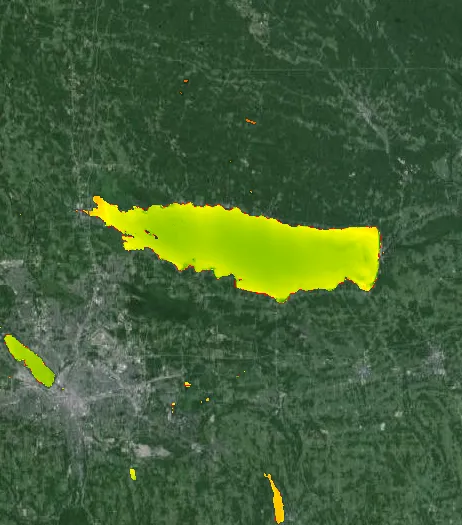
Ross et al. (2019) first proposed using the Water Quality Portal (WQP) (Read et al. (2017)), where organizations can submit surveys of water quality results in the US, along with remotely sensed data, to build water quality measurement models. This study extends Aquasat’s approach by using a bigger timeline and focused geometry using the data from the inland waters of New York State. With more than 10,000 inland water bodies, of which nearly 8000 are lakes, ponds and reservoirs, New York is one of the richest states in terms of freshwater supply (Figure 1). Moreover, restricting the geography to a single state allows us to build models that are more specific to the region and its water bodies since other studies have shown that water quality models are not easily transferable across geographies (Pahlevan et al. (2020), Topp et al. (2021)).

Figure 1:Map of New York State showing all inland water bodies. There are nearly 10,000 inland water bodies in the state of New York, including lakes, ponds, swamps, and reservoirs.
2Data sources
2.1The Water Quality Portal
The Water Quality Portal (WQP) Read et al. (2017) is a collaborative data service developed by the United States Geological Survey (USGS), the Environmental Protection Agency (EPA), and the National Water Quality Monitoring Council (NWQMC). Launched in 2012, the WQP was created to provide a single access point for water quality data collected by federal, state, tribal, and local agencies, as well as non-governmental organizations across the United States. This data is collected using in-situ measurements with probes and lab analytical methods.
The portal aggregates millions of water quality records, including chemical, physical, and biological measurements from rivers, lakes, streams, and other water bodies. By standardizing and integrating data from multiple sources, the WQP enables researchers, policymakers, and the public to easily search, download, and analyze water quality information. This centralized resource supports environmental monitoring, regulatory compliance, scientific research, and informed decision-making related to water resource management. Due to the complexity of data collection and manual steps involved in in-situ sample collection, this data is very infrequent and sometimes unreliable.

Figure 2:Water Quality Portal. https://
2.2Landsat missions
The Landsat program is a series of Earth-observing satellite missions jointly managed by NASA and the US Geological Survey (USGS). Since its inception in 1972, Landsat has provided the longest continuous space-based record of Earth’s land surfaces. The satellites capture multispectral images at regular intervals, enabling the monitoring of environmental changes, land use, agriculture, forestry, and water resources.
Each Landsat satellite is equipped with sensors that detect reflected and emitted energy from the Earth’s surface in visible, near-infrared, and shortwave infrared wavelengths. These data are invaluable for tracking changes in vegetation, surface water, urban development, and natural disasters. The Landsat archive is freely available, making it a critical resource for scientific research and environmental management worldwide. Landsat 7, 8, and 9 missions are Sun-synchronous, near-polar orbit satellites that provide near-global coverage, with a swath-width of nearly 185 km and resolution of 15-100 m. Individually, they have a repeat cycle of 16 days, but when two of these are combined, we get a repeat cycle of 8 days. This allows us to evaluate water quality at any given place on Earth once every 8 days, subject to cloud cover. The revisit times at any given place on Earth are fairly constant.
For water quality studies, Landsat’s spatial and spectral resolution allows for the detection of features such as algal blooms, sediment plumes, and changes in water color, which can be correlated with parameters like Chl-a concentration.

Figure 3:Landsat 9, operational since Sept. 2021, has OLI-2 (visible, NIR, SWIR) and TIRS-2 (thermal) on board.
Source: https://
3Approach
3.1Data curation
This work follows a sequential process of data curation inspired by Ross et al. (2019), with the key objective of matching coincident Landsat data with available WQP measurements for Chl-a in the inland waters of New York State. The entire process is laid out in Figure 4.

Figure 4:A sequential data curation process involves querying data for Chl-a measurements from WQP for New York State’s inland water bodies. This is followed by querying Google Earth Engine (GEE) for corresponding Landsat measurements, filtering our potential sources of noise (cloud cover and pixels around major sources of roads), and matching this data to keep measurements that fall within the major water bodies.
Querying the WQP for Chl-a measurements within the bounds of New York State between January 2015 and October 2023 yields a dataset of 68,075 measurements. WQP is not consistent in its nomenclature and data quality checks, so it was essential to specify different ways of referring to Chl-a. Some of those ways are Chlorophyll, Chlorophyll A, Chlorophyll a, Chlorophyll a (probe relative fluorescence), Chlorophyll a (probe), Chlorophyll a - Periphyton (attached), Chlorophyll a - Phytoplankton (suspended), Chlorophyll a, corrected for pheophytin, and so on. HyRiver, a Python library published by Chegini et al. (2021), was used to connect to the WQP and export data.
To reduce the effect of repeated measurements from the same water body and around the same time, we deduplicate data by removing consecutive values with the same date and time if the relative standard deviation (RSD) of those values was less than 10. Passive remote sensing measurements like Landsat are not sensitive to measuring water quality beyond 100 meters depth. So, we removed all measurements that were reported to be measured beyond 100m in depth. After applying these filters and removing unclean values (where measurement values were not numerical), we are left with 13,717 measurements.
Each record in our WQP dataset is indexed by a unique combination of location (latitude and longitude) and date. For each such unique combination, we query Landsat data to find coincident measurements. We begin by querying Landsat metadata, mainly the scene ID, for each row of our Chl-a WQP dataset. We find all Landsat scenes which included the location of interest and that were imaged within ±1 day of the WQP measurement date using publicly accessible USGS APIs. If no coincident Landsat scenes existed, we discard the measurement. This condition further reduces the number of usable measurements to 8295.
Before querying the actual Landsat data, we further filter out the unnecessary parts from each of these Landsat scenes since we only care about the part that images the area of the water body where the WQP measurement was recorded. We use Google Earth Engine (Gorelick et al. (2017)) to write a data query and pull Landsat imaged data into a tabular featurized form. To do that, we start by creating a 200-meter buffer around the point of interest (WQP measurement location) and removing the region that falls outside this buffer. Next, we remove all bits classified as cloud, cloud shadow, or cirrus. We also remove all pixels within 30 meters of major national roads and rail routes (TIGER Roads data). To ensure we do not inadvertently consider any land pixels in our data, we remove all pixels corresponding to geographies not marked as water with a confidence value of 80% or more in Pekel et al. (2016). 4307 measurements remain after applying all these filters.
Finally, we do a spatial join with the USGS NHD dataset to keep measurements corresponding to lakes, ponds, and reservoirs in NY state with an area of more than 0.005 sq. km but less than 1000 sq. km. That leaves us with 428 readings. Each row in this tabular dataset indicates one reading at a unique location and day. The feature values are surface reflectance from different Landsat bandwidths—Blue, Green, Red, Nir, Swir1, and Swir2.
3.2Statistical modeling
The cleaned dataset of 428 readings was used to train different statistical models with regression—random forest, gradient boosting, Lasso, AdaBoost, and XGBoost. The best model was chosen based on MAE and RMSE scores in a 10-fold cross-validation experiment. The statistical modeling workflow is shown in Figure 5.

Figure 5:Training and cross-validation experiment setup
4Results
4.1Model selection
Based on 10-fold cross-validation results for each algorithm, we find the random forest model performed the best (Table 1) with 500 decision tree estimators. Model algorithm and optimization setup available as part of the scikit-learn project Pedregosa et al., 2011 in Python was used for model training. We choose this model for further inferencing on other Landsat water body scenes with no matching WQP measurements for Chl-a. Figure 6 shows a comparison of the values predicted by this model and the actual Chl-a measurements from WQP.
Table 1:Cross-validation results. The regression metrics shown below are for the best set of hyperparameters for the displayed algorithm.
| Algorithm | RMSE (μg/L) | MAE (μg/L) | R2 (adj.) | MAPE (%) |
|---|---|---|---|---|
| Random forest | 3.18 | 2.22 | 0.90 | 0.93 |
| Gradient boosting | 8.46 | 6.46 | 0.29 | 2.86 |
| Lasso | 9.98 | 7.66 | 0.013 | 3.31 |
| AdaBoost | 8.28 | 6.51 | 0.329 | 3.072 |
| XGBoost | 3.990 | 2.819 | 0.842 | 1.173 |

Figure 6:Values of Chl-a predicted by the best performance model plotted against actual values.
By training models on in-situ WQP data and applying them to Landsat satellite imagery, we can estimate Chlorophyll-a concentrations for over 30 times more locations and days than those directly measured in the WQP dataset. This expanded coverage is shown in Figure 7.

Figure 7:Panel A shows the number of in-situ Chl-a measurements from the Water Quality Portal across New York’s 200 largest lakes between 2015 and 2023. Panel B demonstrates that using remote sensing, we can estimate Chl-a concentrations at over 30 times more locations and dates within the same lakes and time period. Each bubble represents the center of water body and the size of the bubble is proportional to the number of measurements.
5Conclusion
This study demonstrates that combining Landsat satellite imagery with in-situ water quality measurements enables accurate estimation of Chl-a concentration in New York’s inland waters. The curated dataset and rigorous filtering process ensured high-quality training data, and the random forest regression model achieved strong predictive performance. These results highlight the potential of remote sensing and machine learning to supplement traditional water quality monitoring, offering improved spatial and temporal coverage. Future work could expand this approach to other regions and water quality indicators, further supporting environmental management and public health efforts.
Copyright © 2025 Dabhadkar. This is an open-access article distributed under the terms of the Creative Commons Attribution 4.0 International license, which enables reusers to distribute, remix, adapt, and build upon the material in any medium or format, so long as attribution is given to the creator.
- Chl-a
- Chlorophyll-a
- EPA
- Environmental Protection Agency
- GEE
- Google Earth Engine
- HAB
- Harmful Algal Bloom
- MAE
- Mean Absolute Error
- MAPE
- Mean Absolute Percentage Error
- NHD
- National Hydrography Dataset
- NIR
- Near Infrared
- NWQMC
- National Water Quality Monitoring Council
- RMSE
- Root Mean Square Error
- RSD
- relative standard deviation
- SWIR
- Short Wave Infrared
- USGS
- United States Geological Survey
- WQP
- Water Quality Portal
- Karmakar, J., Mondal, I., Hossain, S. A., Jose, F., Pichuka, S., Ghosh, D., De, T. K., Lu, Q.-O., Elkhrachy, I., & Nguyen, N.-M. (2024). Analyzing spatio-temporal variability of aquatic productive components in Northern Bay of Bengal using advanced machine learning models. Ocean & Coastal Management, 251, 107074. 10.1016/j.ocecoaman.2024.107074
- Pahlevan, N., Smith, B., Schalles, J., Binding, C., Cao, Z., Ma, R., Alikas, K., Kangro, K., Gurlin, D., Hà, N., Matsushita, B., Moses, W., Greb, S., Lehmann, M. K., Ondrusek, M., Oppelt, N., & Stumpf, R. (2020). Seamless retrievals of chlorophyll-a from Sentinel-2 (MSI) and Sentinel-3 (OLCI) in inland and coastal waters: A machine-learning approach. Remote Sensing of Environment, 240, 111604. 10.1016/j.rse.2019.111604
- Sahwell, P. J., Bejar, D., Kim, D. M., & Solo-Gabriele, H. M. (2024). Non-traditional abiotic drivers explain variability of chlorophyll-a in a shallow estuarine embayment. Science of The Total Environment, 919, 170873. 10.1016/j.scitotenv.2024.170873
- Ross, M. R. V., Topp, S. N., Appling, A. P., Yang, X., Kuhn, C., Butman, D., Simard, M., & Pavelsky, T. M. (2019). AquaSat: A Data Set to Enable Remote Sensing of Water Quality for Inland Waters. Water Resources Research, 55(11), 10012–10025. 10.1029/2019wr024883
- Read, E. K., Carr, L., De Cicco, L., Dugan, H. A., Hanson, P. C., Hart, J. A., Kreft, J., Read, J. S., & Winslow, L. A. (2017). Water quality data for national‐scale aquatic research: The Water Quality Portal. Water Resources Research, 53(2), 1735–1745. 10.1002/2016wr019993
- Topp, S. N., Pavelsky, T. M., Stanley, E. H., Yang, X., Griffin, C. G., & Ross, M. R. V. (2021). Multi-decadal improvement in US Lake water clarity. Environmental Research Letters, 16(5), 055025. 10.1088/1748-9326/abf002
- Chegini, T., Li, H.-Y., & Leung, L. (2021). HyRiver: Hydroclimate Data Retriever. Journal of Open Source Software, 6(66), 3175. 10.21105/joss.03175
- Gorelick, N., Hancher, M., Dixon, M., Ilyushchenko, S., Thau, D., & Moore, R. (2017). Google Earth Engine: Planetary-scale geospatial analysis for everyone. Remote Sensing of Environment, 202, 18–27. 10.1016/j.rse.2017.06.031
- Pekel, J.-F., Cottam, A., Gorelick, N., & Belward, A. S. (2016). High-resolution mapping of global surface water and its long-term changes. Nature, 540(7633), 418–422. 10.1038/nature20584
- Pedregosa, F., Varoquaux, G., Gramfort, A., Michel, V., Thirion, B., Grisel, O., Blondel, M., Prettenhofer, P., Weiss, R., Dubourg, V., Vanderplas, J., Passos, A., Cournapeau, D., Brucher, M., Perrot, M., & Duchesnay, E. (2011). Scikit-learn: Machine Learning in Python. Journal of Machine Learning Research, 12, 2825–2830. http://jmlr.org/papers/v12/pedregosa11a.html