The myth of the normal curve and what to do about it

Reliance on the normal curve as a tool for measurement is almost a given. It shapes our grading systems, our measures of intelligence, and importantly, it forms the mathematical backbone of many of our inferential statistical tests and algorithms. Some even call it “God’s curve” for its supposed presence in nature Micceri, 1989.

Scientific fields that deal in explanatory and predictive statistics make particular use of the normal curve, often using it to conveniently define thresholds beyond which a result is considered statistically significant (e.g., t-test, F-test). Even familiar machine learning models have, buried in their guts, an assumption of the normal curve (e.g., LDA, gaussian naive Bayes, logistic & linear regression).

The normal curve has had a grip on us for some time; the aphorism by Cramer (1946) still rings true for many today:

“Everyone believes in the [normal] law of errors, the experimenters because they think it is a mathematical theorem, the mathematicians because they think it is an experimental fact.”

Many students of statistics learn that N=40 is enough to ignore the violation of the assumption of normality. This belief stems from early research showing that the sampling distribution of the mean quickly approaches normal, even when drawing from non-normal distributions—as long as samples are sufficiently large. It is common to demonstrate this result by sampling from uniform and exponential distributions. Since these look nothing like the normal curve, it was assumed that N=40 must be enough to avoid practical issues when sampling from other types of non-normal distributions Wilcox, 2013. (Others reached similar conclusions with different methodology Gleason, 1993.)

Two practical issues have since been identified based on this early research: (1) The distributions under study were light tailed (they did not produce outliers), and (2) statistics other than the sample mean were not tested and may behave differently. In the half century following these early findings, many important discoveries have been made—calling into question the usefulness of the normal curve Wilcox, 2013.

The following sections uncover various pitfalls one might encounter when assuming normality—especially as they relate to hypothesis testing. To help researchers overcome these problems, a new Python library for robust hypothesis testing will be introduced along with an interactive tool for robust statistics education.

The contaminated normal¶

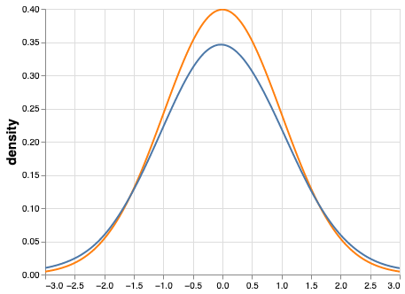
One of the most striking counterexamples of “N=40 is enough” is shown when sampling from the so-called contaminated normal Tukey, 1960Tan, 1982. This distribution is also bell shaped and symmetrical but it has slightly heavier tails when compared to the standard normal curve. That is, it contains outliers and is difficult to distinguish from a normal distribution with the naked eye. Consider the distributions in Figure 1. The variance of the normal distribution is 1 but the variance of the contaminated normal is 10.9!

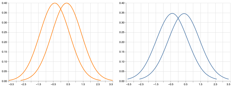
The consequence of this inflated variance is apparent when examining statistical power. To demonstrate, Figure 2 shows two pairs of distributions: On the left, there are two normal distributions (variance 1) and on the right there are two contaminated distributions (variance 10.9). Both pairs of distributions have a mean difference of 0.8. Wilcox (2013) showed that by taking random samples of N=40 from each normal curve, and comparing them with Student’s t-test, statistical power was approximately 0.94. However, when following this same procedure for the contaminated groups, statistical power was only 0.25.

The point here is that even small apparent departures from normality, especially in the tails, can have a large impact on commonly used statistics. The problems continue to get worse when examining effect sizes but these findings are not discussed in this article. Interested readers should see Wilcox’s 1992 paper Wilcox, 1992.

Perhaps one could argue that the contaminated normal distribution actually represents an extreme departure from normality and therefore should not be taken seriously; however, distributions that generate outliers are likely common in practice Hill & Dixon, 1982Micceri, 1989Wilcox, 2009. A reasonable goal would then be to choose methods that perform well under such situations and continue to perform well under normality. In addition, serious issues still exist even when examining light-tailed and skewed distributions (e.g., lognormal), and statistics other than the sample mean (e.g., T). These findings will be discussed in the following section.

Student’s t-distribution¶

Another common statistic is the T value obtained from Student’s t-test. As will be demonstrated, T is more sensitive to violations of normality than the sample mean (which has already been shown to not be robust). This is despite the fact that the t-distribution is also bell shaped, light tailed, and symmetrical—a close relative of the normal curve.

The assumption is that T follows a t-distribution (and with large samples it approaches normality). We can test this assumption by generating random samples from a lognormal distribution. Specifically, 5000 datasets of sample size 20 were randomly drawn from a lognormal distribution using SciPy’s lognorm.rvs function. For each dataset, T was calculated and the resulting t-distribution was plotted. 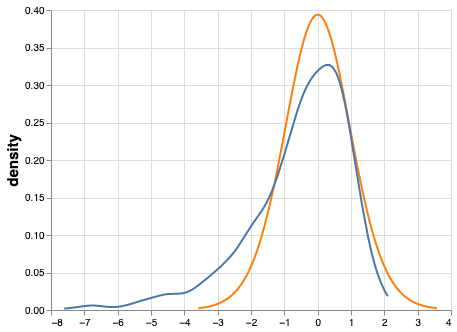Figure 3 shows that the assumption that T follows a t-distribution does not hold.

With N=20, the assumption is that with a probability of 0.95, T will be between -2.09 and 2.09. However, when sampling from a lognormal distribution in the manner just described, there is actually a 0.95 probability that T will be between approximately -4.2 and 1.4 (i.e., the middle 95% of the actual t-distribution is much wider than the assumed t-distribution). Based on this result we can conclude that sampling from skewed distributions (e.g., lognormal) leads to increased Type I Error when using Student’s t-test Wilcox, 1998.

Modern robust methods¶

When it comes to hypothesis testing, one intuitive way of dealing with the issues described above would be to (1) replace the sample mean (and standard deviation) with a robust alternative and (2) use a non-parametric resampling technique to estimate the sampling distribution (rather than assuming a theoretical shape) ^[1]. Two such candidates are the 20% trimmed mean and the percentile bootstrap test, both of which have been shown to have practical value when dealing with issues of outliers and non-normality Campopiano et al., 2018Wilcox, 2013.

The trimmed mean¶

The trimmed mean is nothing more than sorting values, removing a proportion from each tail, and computing the mean on the remaining values. Formally,

• Let $X_1 ... X_n$ be a random sample and $X_{(1)} \leq X_{(2)} ... \leq X_{(n)}$ be the observations in ascending order
• The proportion to trim is $\gamma (0 \leq \gamma \leq .5)$
• Let $g = \lfloor \gamma n \rfloor$. That is, the proportion to trim multiplied by $n$, rounded down to the nearest integer

Then, in symbols, the trimmed mean can be expressed as follows:

If the proportion to trim is 0.2, more than twenty percent of the values would have to be altered to make the trimmed mean arbitrarily large or small. The sample mean, on the other hand, can be made to go to $\pm\infty$ (arbitrarily large or small) by changing a single value. The trimmed mean is more robust than the sample mean in all measures of robustness that have been studied Wilcox, 2013. In particular the 20% trimmed mean has been shown to have practical value as it avoids issues associated with the median (not discussed here) and still protects against outliers.

The percentile bootstrap test¶

In most traditional parametric tests, there is an assumption that the sampling distribution has a particular shape (normal, f-distribution, t-distribution, etc). We can use these distributions to test the null hypothesis; however, as discussed, the theoretical distributions are not always approximated well when violations of assumptions occur. Non-parametric resampling techniques such as bootstrapping and permutation tests build empirical sampling distributions, and from these, one can robustly derive p-values and CIs. One example is the percentile bootstrap test Efron, 1992Tibshirani & Efron, 1993.

The percentile bootstrap test can be thought of as an algorithm that uses the data at hand to estimate the underlying sampling distribution of a statistic (pulling yourself up by your own bootstraps, as the saying goes). This approach is in contrast to traditional methods that assume the sampling distribution takes a particular shape). The percentile boostrap test works well with small sample sizes, under normality, under non-normality, and it easily extends to multi-group tests (ANOVA) and measures of association (correlation, regression). For a two-sample case, the steps to compute the percentile bootstrap test can be described as follows:

1. Randomly resample with replacement $n$ values from group one
2. Randomly resample with replacement $n$ values from group two
3. Compute $\bar{X}_1 - \bar{X}_2$ based on you new sample (the mean difference)
4. Store the difference & repeat steps 1-3 many times (say, 1000)
5. Consider the middle 95% of all differences (the confidence interval)
6. If the confidence interval contains zero, there is no statistical difference, otherwise, you can reject the null hypothesis (there is a statistical difference)

Implementing and teaching modern robust methods¶

Despite over a half a century of convincing findings, and thousands of papers, robust statistical methods are still not widely adopted in applied research Erceg-Hurn & Mirosevich, 2008Wilcox, 1998. This may be due to various false beliefs. For example,

• Classical methods are robust to violations of assumptions
• Correcting non-normal distributions by transforming the data will solve all issues
• Traditional non-parametric tests are suitable replacements for parametric tests that violate assumptions

Perhaps the most obvious reason for the lack of adoption of modern methods is a lack of easy-to-use software and training resources. In the following sections, two resources will be presented: one for implementing robust methods and one for teaching them.

Robust statistics for Python¶

Hypothesize is a robust null hypothesis significance testing (NHST) library for Python Campopiano & Wilcox, 2020. It is based on Wilcox’s WRS package for R which contains hundreds of functions for computing robust measures of central tendency and hypothesis testing. At the time of this writing, the WRS library in R contains many more functions than Hypothesize and its value to researchers who use inferential statistics cannot be understated. WRS is best experienced in tandem with Wilcox’s book “Introduction to Robust Estimation and Hypothesis Testing”.

Hypothesize brings many of these functions into the open-source Python library ecosystem with the goal of lowering the barrier to modern robust methods—even for those who have not had extensive training in statistics or coding. With modern browser-based notebook environments (e.g., Deepnote), learning to use Hypothesize can be relatively straightforward. In fact, every statistical test listed in the docs is associated with a hosted notebook, pre-filled with sample data and code. But certainly, simply pip install Hypothesize to use Hypothesize in any environment that supports Python. See Noordt & Willoughby (2021) and Noordt et al. (2022) for examples of Hypothesize being used in applied research.

The API for Hypothesize is organized by single- and two-factor tests, as well as measures of association. Input data for the groups, conditions, and measures are given in the form of a Pandas DataFrame team, 2020McKinney, 2010. By way of example, one can compare two independent groups (e.g., placebo versus treatment) using the 20% trimmed mean and the percentile bootstrap test, as follows (note that Hypothesize uses the naming conventions found in WRS):

from hypothesize.utilities import trim_mean
from hypothesize.compare_groups_with_single_factor \
    import pb2gen

results = pb2gen(df.placebo, df.treatment, trim_mean)

As shown below, the results are returned as a Python dictionary containing the p-value, confidence intervals, and other important details.

{
'ci': [-0.22625614592148624, 0.06961754796950131],
'est_1': 0.43968438076483285,
'est_2': 0.5290985245430996,
'est_dif': -0.08941414377826673,
'n1': 50,
'n2': 50,
'p_value': 0.27,
'variance': 0.005787027326924963
}

For measuring associations, several options exist in Hypothesize. One example is the Winsorized correlation which is a robust alternative to Pearson’s R. For example,

from hypothesize.measuring_associations import wincor

results = wincor(df.height, df.weight, tr=.2)

returns the Winsorized correlation coefficient and other relevant statistics:

{
'cor': 0.08515087411576182,
'nval': 50,
'sig': 0.558539575073185,
'wcov': 0.004207827245660796
}

A case study using real-world data¶

It is helpful to demonstrate that robust methods in Hypothesize (and in other libraries) can make a practical difference when dealing with real-world data. In a study by Miller on sexual attitudes, 1327 men and 2282 women were asked how many sexual partners they desired over the next 30 years (the data are available from Rand R. Wilcox’s site). When comparing these groups using Student’s t-test, we get the following results:

{
'ci': [-1491.09,  4823.24],
't_value': 1.035308,
'p_value': 0.300727
}

That is, we fail to reject the null hypothesis at the $\alpha=0.05$ level using Student’s test for independent groups. However, if we switch to a robust analogue of the t-test, one that utilizes bootstrapping and trimmed means, we can indeed reject the null hypothesis. Here are the corresponding results from Hypothesize’s yuenbt test (based on Yuen (1974)):

from hypothesize.compare_groups_with_single_factor \
    import yuenbt

results = yuenbt(df.males, df.females,
    tr=.2, alpha=.05)

{
'ci': [1.41, 2.11],
'test_stat': 9.85,
'p_value': 0.0
}

The point here is that robust statistics can make a practical difference with real-world data (even when N is considered large). Many other examples of robust statistics making a practical difference with real-world data have been documented Hill & Dixon, 1982Wilcox, 2009Wilcox, 2001.

It is important to note that robust methods may also fail to reject when a traditional test rejects (remember that traditional tests can suffer from increased Type I Error). It is also possible that both approaches yield the same or similar conclusions. The exact pattern of results depends largely on the characteristics of the underlying population distribution. To be able to reason about how robust statistics behave when compared to traditional methods the robust statistics simulator has been created and is described in the next section.

Robust statistics simulator¶

Having a library of robust statistical functions is not enough to make modern methods commonplace in applied research. Educators and practitioners still need intuitive training tools that demonstrate the core issues surrounding classical methods and how robust analogues compare.

As mentioned, computational notebooks that run in the cloud offer a unique solution to learning beyond that of static textbooks and documentation. Learning can be interactive and exploratory since narration, visualization, widgets (e.g., buttons, slider bars), and code can all be experienced in a ready-to-go compute environment—with no overhead related to local environment setup.

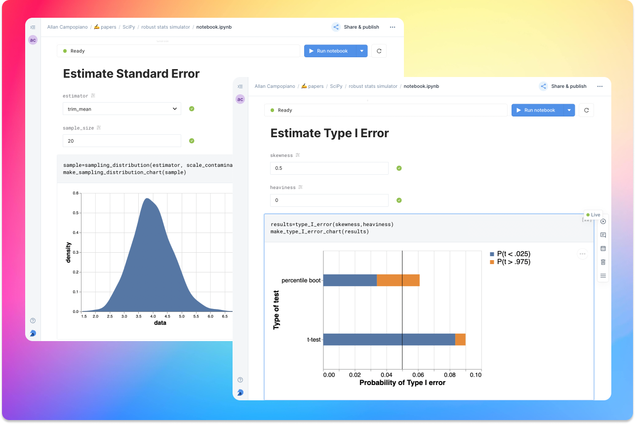
As a compendium to Hypothesize, and a resource for understanding and teaching robust statistics in general, the robust statistics simulator repository has been developed. It is a notebook-based collection of interactive demonstrations aimed at clearly and visually explaining the conditions under which classic methods fail relative to robust methods. A hosted notebook with the rendered visualizations of the simulations can be accessed here and seen in Figure 4. Since the simulations run in the browser and require very little understanding of code, students and teachers can easily onboard to the study of robust statistics.

The robust statistics simulator allows users to interact with the following parameters:

• Distribution shape
• Level of contamination
• Sample size
• Skew and heaviness of tails

Each of these characteristics can be adjusted independently in order to compare classic approaches to their robust alternatives. The two measures that are used to evaluate the performance of classic and robust methods are the standard error and Type I Error.

Standard error is a measure of how much an estimator varies across random samples from our population. We want to choose estimators that have a low standard error. Type I Error is also known as False Positive Rate. We want to choose methods that keep Type I Error close to the nominal rate (usually 0.05). The robust statistics simulator can guide these decisions by providing empirical evidence as to why particular estimators and statistical tests have been chosen.

Conclusion¶

This paper gives an overview of the issues associated with the normal curve. The concern with traditional methods, in terms of robustness to violations of normality, have been known for over a half century and modern alternatives have been recommended; however, for various reasons that have been discussed, modern robust methods have not yet become commonplace in applied research settings.

One reason is the lack of easy-to-use software and teaching resources for robust statistics. To help fill this gap, Hypothesize, a peer-reviewed and open-source Python library was developed. In addition, to help clearly demonstrate and visualize the advantages of robust methods, the robust statistics simulator was created. Using these tools, practitioners can begin to integrate robust statistical methods into their inferential testing repertoire.