
Bayesian Estimation and Forecasting of Time Series in statsmodels
Abstract
Statsmodels, a Python library for statistical and econometric analysis,
has traditionally focused on frequentist inference, including in its
models for time series data. This paper introduces the powerful features
for Bayesian inference of time series models that exist in statsmodels, with
applications to model fitting, forecasting, time series decomposition,
data simulation, and impulse response functions.
Introduction
Statsmodels Seabold & Perktold, 2010 is a well-established Python
library for statistical and econometric analysis, with support for a wide range
of important model classes, including linear regression, ANOVA, generalized
linear models (GLM), generalized additive models (GAM), mixed effects models,
and time series models, among many others. In most cases, model fitting proceeds
by using frequentist inference, such as maximum likelihood estimation (MLE). In
this paper, we focus on the class of time series models
McKinney et al., 2011, support for which has grown substantially in
statsmodels over the last decade. After introducing several of the most
important new model classes – which are by default fitted using MLE – and
their features – which include forecasting, time series decomposition and
seasonal adjustment, data simulation, and impulse response analysis – we
describe the powerful functions that enable users to apply Bayesian methods to
a wide range of time series models.
Support for Bayesian inference in Python outside of statsmodels has also grown
tremendously, particularly in the realm of probabilistic programming, and
includes powerful libraries such as
PyMC3 Salvatier et al., 2016, PyStan Carpenter et al., 2017,
and TensorFlow Probability Dillon et al., 2017. Meanwhile,
ArviZ Kumar et al., 2019 provides many excellent tools for associated
diagnostics and vizualisations. The aim of these libraries is to provide support
for Bayesian analysis of a large class of models, and they make available both
advanced techniques, including auto-tuning algorithms, and flexible model
specification. By contrast, here we focus on simpler techniques. However, while
the libraries above do include some support for time series models, this has not
been their primary focus. As a result, introducing Bayesian inference for the
well-developed stable of time series models in statsmodels, and providing
access to the rich associated feature set already mentioned, presents a
complementary option to these more general-purpose libraries.[1]
Time series analysis in statsmodels
A time series is a sequence of observations ordered in time, and time series data appear commonly in statistics, economics, finance, climate science, control systems, and signal processing, among many other fields. One distinguishing characteristic of many time series is that observations that are close in time tend to be more correlated, a feature known as autocorrelation. While successful analyses of time series data must account for this, statistical models can harness it to decompose a time series into trend, seasonal, and cyclical components, produce forecasts of future data, and study the propagation of shocks over time.
We now briefly review the models for time series data that are available in
statsmodels and describe their features.[2]
Exponential smoothing models
Exponential smoothing models are constructed by combining one or more simple equations that each describe some aspect of the evolution of univariate time series data. While originally somewhat ad hoc, these models can be defined in terms of a proper statistical model (for example, see Hyndman et al. (2008)). They have enjoyed considerable popularity in forecasting (for example, see the implementation in R described by Hyndman & Athanasopoulos (2018)). A prototypical example that allows for trending data and a seasonal component – often known as the additive “Holt-Winters’ method” – can be written as
where is the level of the series, is the trend,
is the seasonal component of period , and
are parameters of the model. When augmented with
an error term with some given probability distribution (usually Gaussian),
likelihood-based inference can be used to estimate the parameters.
In statsmodels, additive exponential smoothing models
can be constructed using the statespace.ExponentialSmoothing class.[3]
The following code shows how to apply the additive Holt-Winters model above to
model quarterly data on consumer prices:
import statsmodels.api as sm
# Load data
mdata = sm.datasets.macrodata.load().data
# Compute annualized consumer price inflation
y = np.log(mdata['cpi']).diff().iloc[1:] * 400

# Construct the Holt-Winters model
model_hw = sm.tsa.statespace.ExponentialSmoothing(
   y, trend=True, seasonal=12)
Structural time series models
Structural time series models, introduced by Harvey (1990) and also sometimes known as unobserved components models, similarly decompose a univariate time series into trend, seasonal, cyclical, and irregular components:
where is the trend, is the seasonal component,
is the cyclical component, and
is the error term. However, this
equation can be augmented in many ways, for example to include explanatory
variables or an autoregressive component. In addition, there are many possible
specifications for the trend, seasonal, and cyclical components, so that a wide
variety of time series characteristics can be accommodated. In statsmodels,
these models can be constructed from the UnobservedComponents class; a
few examples are given in the following code:
# "Local level" model
model_ll = sm.tsa.UnobservedComponents(y, 'llevel')
# "Local linear trend", with seasonal component
model_arma11 = sm.tsa.UnobservedComponents(
   y, 'lltrend', seasonal=4)
These models have become popular for time series analysis and forecasting, as they are flexible and the estimated components are intuitive. Indeed, Google’s Causal Impact library Brodersen et al., 2015 uses a Bayesian structural time series approach directly, and Facebook’s Prophet library Taylor & Letham, 2017 uses a conceptually similar framework and is estimated using PyStan.
Autoregressive moving-average models
Autoregressive moving-average (ARMA) models, ubiquitous in time series
applications, are well-supported in statsmodels, including their
generalizations, abbreviated as “SARIMAX”, that allow for integrated time series
data, explanatory variables, and seasonal effects.[4] A general version of
this model, excluding integration, can be written as
where . These are constructed in
statsmodels with the ARIMA class; the following code shows how to
construct a variety of autoregressive moving-average models for consumer price
data:
# AR(2) model
model_ar2 = sm.tsa.ARIMA(y, order=(2, 0, 0))
# ARMA(1, 1) model with explanatory variable
X = mdata['realint']
model_arma11 = sm.tsa.ARIMA(
   y, order=(1, 0, 1), exog=X)
# SARIMAX(p, d, q)x(P, D, Q, s) model
model_sarimax = sm.tsa.ARIMA(
   y, order=(p, d, q), seasonal_order=(P, D, Q, s))
While this class of models often produces highly competitive forecasts, it does not produce a decomposition of a time series into, for example, trend and seasonal components.
Vector autoregressive models
While the SARIMAX models above handle univariate series, statsmodels also has
support for the multivariate generalization to vector autoregressive (VAR)
models.[5] These models are written
where is now considered as an vector. As a result,
the intercept ν is also an vector, the
coefficients are each matrices, and the error
term is , with Ω an
matrix. These models can be constructed in statsmodels
using the VARMAX class, as follows[6]
# Multivariate dataset
z = (np.log(mdata['realgdp', 'realcons', 'cpi'])
       .diff().iloc[1:])

# VAR(1) model
model_var = sm.tsa.VARMAX(z, order=(1, 0))
Dynamic factor models
statsmodels also supports a second model for multivariate time series: the
dynamic factor model (DFM). These models, often used for dimension reduction,
posit a few unobserved factors, with autoregressive dynamics, that are used to
explain the variation in the observed dataset. In statsmodels, there are two
model classes, DynamicFactor and DynamicFactorMQ, that can fit
versions of the DFM. Here we focus on the DynamicFactor class, for which
the model can be written
Here again, the observation is assumed to be , but the factors are , where it is possible that . As before, we assume conformable coefficient matrices and Gaussian errors.
The following code shows how to construct a DFM in statsmodels
# DFM with 2 factors that evolve as a VAR(3)
model_dfm = sm.tsa.DynamicFactor(
   z, k_factors=2, factor_order=3)
Linear Gaussian state space models

Figure 1:Selected functionality of state space models in statsmodels.
In statsmodels, each of the model classes introduced above (
statespace.ExponentialSmoothing, UnobservedComponents,
ARIMA, VARMAX, DynamicFactor, and
DynamicFactorMQ) are implemented as part of a broader class of models,
referred to as linear Gaussian state space models (hereafter for brevity, simply
“state space models” or SSM). This class of models can be written as
where represents an unobserved vector containing the “state” of the dynamic system. In general, the model is multivariate, with and vector, , and .
Powerful tools exist for state space models to estimate the
values of the unobserved state vector, compute the value of the likelihood
function for frequentist inference, and perform posterior sampling for Bayesian
inference. These tools include the celebrated Kalman filter and smoother and
a simulation smoother, all of which are important for conducting Bayesian
inference for these models.[7] The implementation in statsmodels largely follows
the treatment in Durbin & Koopman (2012), and is described in more detail in
Fulton (2015).
In addition to these key tools, state space models also admit general implementations of useful features such as forecasting, data simulation, time series decomposition, and impulse response analysis. As a consequence, each of these features extends to each of the time series models described above. Figure 1 presents a diagram showing how to produce these features, and the code below briefly introduces a subset of them.
# Construct the Model
model_ll = sm.tsa.UnobservedComponents(y, 'llevel')

# Construct a simulation smoother
sim_ll = model_ll.simulation_smoother()

# Parameter values (variance of error and
# variance of level innovation, respectively)
params = [4, 0.75]

# Compute the log-likelihood of these parameters
llf = model_ll.loglike(params)

# `smooth` applies the Kalman filter and smoother
# with a given set of parameters and returns a
# Results object
results_ll = model_ll.smooth(params)

# Produce forecasts for the next 4 periods
fcast = results_ll.forecast(4)

# Produce a draw from the posterior distribution
# of the state vector
sim_ll.simulate()
draw = sim_ll.simulated_state
Nearly identical code could be used for any of the model classes introduced above, since they are all implemented as part of the same state space model framework. In the next section, we show how these features can be used to perform Bayesian inference with these models.
Bayesian inference via Markov chain Monte Carlo
We begin by giving a cursory overview of the key elements of Bayesian inference required for our purposes here.[8] In brief, the Bayesian approach stems from Bayes’ theorem, in which the posterior distribution for an object of interest is derived as proportional to the combination of a prior distribution and the likelihood function
Here, we will be interested in the posterior distribution of the parameters
of our model and of the unobserved states, conditional on the chosen model
specification and the observed time series data. While in most cases the form
of the posterior cannot be derived analytically, simulation-based methods such
as Markov chain Monte Carlo (MCMC) can be used to draw samples that approximate
the posterior distribution nonetheless. While PyMC3, PyStan, and TensorFlow
Probability emphasize Hamiltonian Monte Carlo (HMC) and no-U-turn sampling
(NUTS) MCMC methods, we focus on the simpler random walk Metropolis-Hastings
(MH) and Gibbs sampling (GS) methods. These are standard MCMC methods that
have enjoyed great success in time series applications and which are simple to
implement, given the state space framework already available in statsmodels.
In addition, the ArviZ library is designed to work with MCMC output from any
source, and we can easily adapt it to our use.
With either Metropolis-Hastings or Gibbs sampling, our procedure will produce a sequence of sample values (of parameters and / or the unobserved state vector) that approximate draws from the posterior distribution arbitrarily well, as the number of length of the chain of samples becomes very large.
Random walk Metropolis-Hastings
In random walk Metropolis-Hastings (MH), we begin with an arbitrary point as the initial sample, and then iteratively construct new samples in the chain as follows. At each iteration, (a) construct a proposal by perturbing the previous sample by a Gaussian random variable, and then (b) accept the proposal with some probability. If a proposal is accepted, it becomes the next sample in the chain, while if it is rejected then the previous sample value is carried over. Here, we show how to implement Metropolis-Hastings estimation of the variance parameter in a simple model, which only requires the use of the log-likelihood computation introduced above.
import arviz as az
from scipy import stats

# Construct the model
model_rw = sm.tsa.UnobservedComponents(y, 'rwalk')

# Specify the prior distribution. With MH, this
# can be freely chosen by the user
prior = stats.uniform(0.0001, 100)

# Specify the Gaussian perturbation distribution
perturb = stats.norm(scale=0.1)

# Storage
niter = 100000
samples_rw = np.zeros(niter + 1)

# Initialization
samples_rw[0] = y.diff().var()
llf = model_rw.loglike(samples_rw[0])
prior_llf = prior.logpdf(samples_rw[0])

# Iterations
for i in range(1, niter + 1):
   # Compute the proposal value
   proposal = samples_rw[i - 1] + perturb.rvs()

   # Compute the acceptance probability
   proposal_llf = model_rw.loglike(proposal)
   proposal_prior_llf = prior.logpdf(proposal)
   accept_prob = np.exp(
      proposal_llf - llf
      + prior_llf - proposal_prior_llf)

   # Accept or reject the value
   if accept_prob > stats.uniform.rvs():
      samples_rw[i] = proposal
      llf = proposal_llf
      prior_llf = proposal_prior_llf
   else:
      samples_rw[i] = samples_rw[i - 1]

# Convert for use with ArviZ and plot posterior
samples_rw = az.convert_to_inference_data(
   samples_rw)
# Eliminate the first 10000 samples as burn-in;
# thin by factor of 10 to reduce autocorrelation
az.plot_posterior(samples_rw.posterior.sel(
   {'draw': np.s_[10000::10]}), kind='bin',
   point_estimate='median')
Figure 2:Approximate posterior distribution of variance parameter, random walk model, Metropolis-Hastings; U.S. Industrial Production.
The approximate posterior distribution, constructed from the sample chain, is shown in Figure 2.
Gibbs sampling
Gibbs sampling (GS) is a special case of Metropolis-Hastings (MH) that is applicable when it is possible to produce draws directly from the conditional distributions of every variable, even though it is still not possible to derive the general form of the joint posterior. While this approach can be superior to random walk MH when it is applicable, the ability to derive the conditional distributions typically requires the use of a “conjugate” prior – i.e., a prior from some specific family of distributions. For example, above we specified a uniform distribution as the prior when sampling via MH, but that is not possible with Gibbs sampling. Here, we show how to implement Gibbs sampling estimation of the variance parameter, now making use of an inverse Gamma prior, and the simulation smoother introduced above.

Figure 3:Approximate posterior joint distribution of variance parameters, local level model, Gibbs sampling; CPI inflation.
# Construct the model and simulation smoother
model_ll = sm.tsa.UnobservedComponents(y, 'llevel')
sim_ll = model_ll.simulation_smoother()

# Specify the prior distributions. With GS, we must
# choose an inverse Gamma prior for each variance
priors = [stats.invgamma(0.01, scale=0.01)] * 2

# Storage
niter = 100000
samples_ll = np.zeros((niter + 1, 2))

# Initialization
samples_ll[0] = [y.diff().var(), 1e-5]

# Iterations
for i in range(1, niter + 1):
   # (a) Update the model parameters
   model_ll.update(samples_ll[i - 1])

   # (b) Draw from the conditional posterior of
   # the state vector
   sim_ll.simulate()
   sample_state = sim_ll.simulated_state.T

   # (c) Compute / draw from conditional posterior
   # of the parameters:
   # ...observation error variance
   resid = y - sample_state[:, 0]
   post_shape = len(resid) / 2 + 0.01
   post_scale = np.sum(resid**2) / 2 + 0.01
   samples_ll[i, 0] = stats.invgamma(
      post_shape, scale=post_scale).rvs()

   # ...level error variance
   resid = sample_state[1:] - sample_state[:-1]
   post_shape = len(resid) / 2 + 0.01
   post_scale = np.sum(resid**2) / 2 + 0.01
   samples_ll[i, 1] = stats.invgamma(
      post_shape, scale=post_scale).rvs()

# Convert for use with ArviZ and plot posterior
samples_ll = az.convert_to_inference_data(
   {'parameters': samples_ll[None, ...]},
   coords={'parameter': model_ll.param_names},
   dims={'parameters': ['parameter']})
az.plot_pair(samples_ll.posterior.sel(
   {'draw': np.s_[10000::10]}), kind='hexbin');
The approximate posterior distribution, constructed from the sample chain, is shown in Figure 3.
Illustrative examples
For clarity and brevity, the examples in the previous section gave results for simple cases. However, these basic methods carry through to each of the models introduced earlier, including in cases with multivariate data and hundreds of parameters. Moreover, the Metropolis-Hastings approach can be combined with the Gibbs sampling approach, so that if the end user wishes to use Gibbs sampling for some parameters, they are not restricted to choose only conjugate priors for all parameters.
In addition to sampling the posterior distributions of the parameters, this method allows sampling other objects of interest, including forecasts of observed variables, impulse response functions, and the unobserved state vector. This last possibility is especially useful in cases such as the structural time series model, in which the unobserved states correspond to interpretable elements such as the trend and seasonal components. We provide several illustrative examples of the various types of analysis that are possible.
Forecasting and Time Series Decomposition

Figure 4:Data and forecast with 80% credible interval; U.S. Industrial Production.
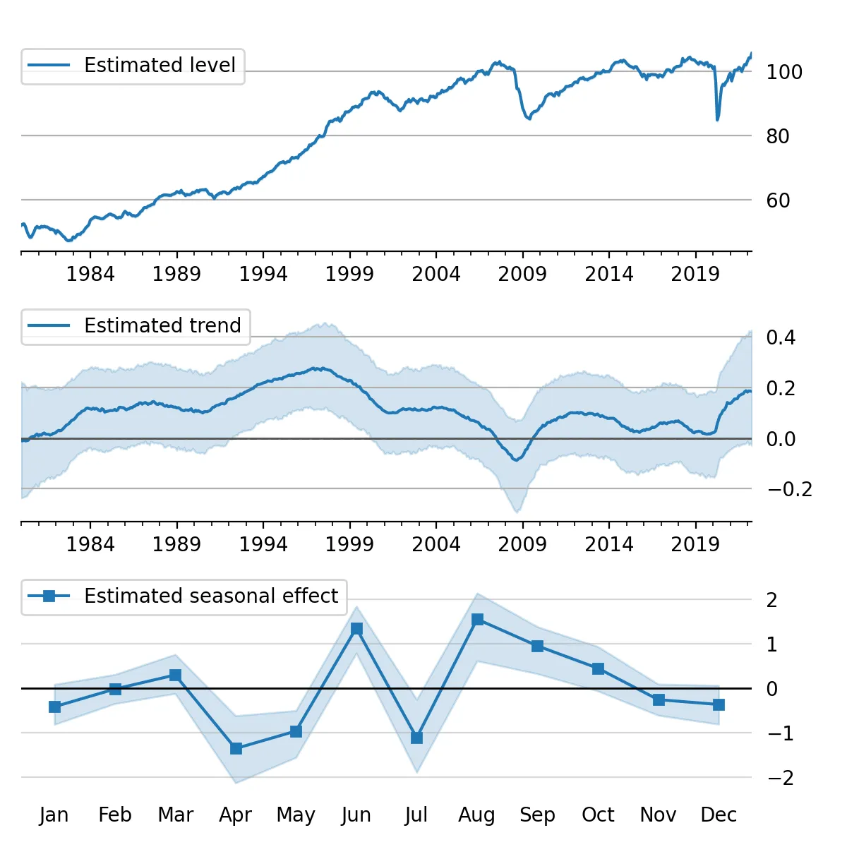
Figure 5:Estimated level, trend, and seasonal components, with 80% credible interval; U.S. Industrial Production.
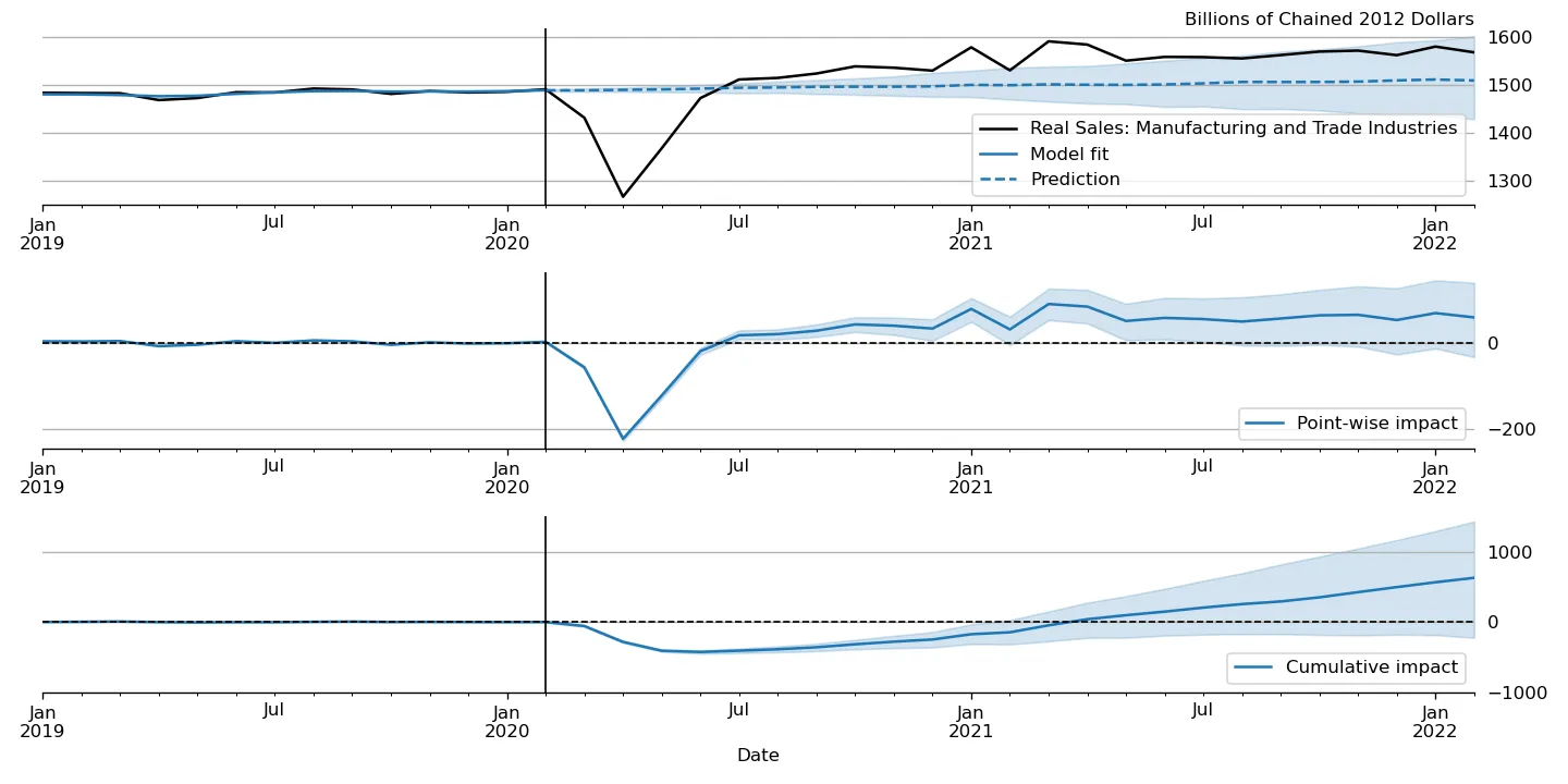
Figure 6:“Causal impact” of COVID-19 on U.S. Sales in Manufacturing and Trade Industries.
In our first example, we apply the Gibbs sampling approach to a structural time series model in order to forecast U.S. Industrial Production and to produce a decomposition of the series into level, trend, and seasonal components. The model is
Here, we set the seasonal periodicity to s=12, since Industrial Production is
a monthly variable. We can construct this model in Statsmodels as[9]
model = sm.tsa.UnobservedComponents(
   y, 'lltrend', seasonal=12)
To produce the time-series decomposition into level, trend, and seasonal
components, we will use samples from the posterior of the state vector
for each time period . These are
immediately available when using the Gibbs sampling approach; in the earlier
example, the draw at each iteration was assigned to the variable sample_state.
To produce forecasts, we need to draw from the posterior predictive
distribution for horizons . This can
be easily accomplished by using the simulate method introduced earlier. To be
concrete, we can accomplish these tasks by modifying section (b) of our Gibbs
sampler iterations as follows:
# (b') Draw from the conditional posterior of
# the state vector
model.update(params[i - 1])
sim.simulate()
# save the draw for use later in time series
# decomposition
states[i] = sim.simulated_state.T

# Draw from the posterior predictive distribution
# using the `simulate` method
n_fcast = 48
fcast[i] = model.simulate(
   params[i - 1], n_fcast,
   initial_state=states[i, -1]).to_frame()
These forecasts and the decomposition into level, trend, and seasonal components are summarized in Figure 4 and Figure 5, which show the median values along with 80% credible intervals. Notably, the intervals shown incorporate for both the uncertainty arising from the stochastic terms in the model as well as the need to estimate the models’ parameters.[10]
Casual impacts
A closely related procedure described in Brodersen et al. (2015) uses a Bayesian structural time series model to estimate the “causal impact” of some event on some observed variable. This approach stops estimation of the model just before the date of an event and produces a forecast by drawing from the posterior predictive density, using the procedure described just above. It then uses the difference between the actual path of the data and the forecast to estimate impact of the event.
An example of this approach is shown in Figure 6, in which we use this method to illustrate the effect of the COVID-19 pandemic on U.S. Sales in Manufacturing and Trade Industries.[11]
Extensions
There are many extensions to the time series models presented here that are
made possible when using Bayesian inference. First, it is easy to create custom
state space models within the statsmodels framework. As one example, the
statsmodels documentation describes how to create a model that extends the
typical VAR described above with time-varying parameters.[12] These custom
state space models automatically inherit all the functionality described above,
so that Bayesian inference can be conducted in exactly the same way.
Second, because the general state space model available in statsmodels and
introduced above allows for time-varying system matrices, it is possible using
Gibbs sampling methods to introduce support for automatic outlier handling,
stochastic volatility, and regime switching models, even though these are
largely infeasible in statsmodels when using frequentist methods such as
maximum likelihood estimation.[13]
Conclusion
This paper introduces the suite of time series models available in statsmodels
and shows how Bayesian inference using Markov chain Monte Carlo methods can be
applied to estimate their parameters and produce analyses of interest, including
time series decompositions and forecasts.
Copyright © 2022 Fulton. This is an open-access article distributed under the terms of the Creative Commons Attribution 3.0 Unported license.
In addition, it is possible to combine the sampling algorithms of PyMC3 with the time series models of
statsmodels, although we will not discuss this approach in detail here. See, for example, https://www .statsmodels .org /v0 .13 .0 /examples /notebooks /generated /statespace _sarimax _pymc3 .html. In addition to statistical models,
statsmodelsalso provides a number of tools for exploratory data analysis, diagnostics, and hypothesis testing related to time series data; see https://www .statsmodels .org /stable /tsa .html. A second class,
ETSModel, can also be used for both additive and multiplicative models, and can exhibit superior performance with maximum likelihood estimation. However, it lacks some of the features relevant for Bayesian inference discussed in this paper.Note that in
statsmodels, models with explanatory variables are in the form of “regression with SARIMA errors”.statsmodelsalso supports vector moving-average (VMA) models using the same model class as described here for the VAR case, but, for brevity, we do not explicitly discuss them here.A second class,
VAR, can also be used to fit VAR models, using least squares. However, it lacks some of the features relevant for Bayesian inference discussed in this paper.Statsmodelscurrently contains two implementations of simulation smoothers for the linear Gaussian state space model. The default is the “mean correction” simulation smoother of Durbin & Koopman (2002). The precision-based simulation smoother of Chan & Jeliazkov (2009) can alternatively be used by specifyingmethod='cfa'when creating the simulation smoother object.While a detailed description of these issues is out of the scope of this paper, there are many superb references on this topic. We refer the interested reader to West & Harrison (1999), which provides a book-length treatment of Bayesian inference for state space models, and Kim & Nelson (1999), which provides many examples and applications.
This model is often referred to as a “local linear trend” model (with additionally a seasonal component);
lltrendis an abbreviation of this name.The popular Prophet library, Taylor & Letham (2017), similarly uses an additive model combined with Bayesian sampling methods to produce forecasts and decompositions, although its underlying model is a GAM rather than a state space model.
In this example, we used a local linear trend model with no seasonal component.
See, for example, Stock & Watson (2016) for an application of these techniques that handles outliers, Kim et al. (1998) for stochastic volatility, and Kim & Nelson (1998) for an application to dynamic factor models with regime switching.
- ARMA
- autoregressive moving-average
- DFM
- dynamic factor model
- GAM
- generalized additive models
- GLM
- generalized linear models
- GS
- Gibbs sampling
- HMC
- Hamiltonian Monte Carlo
- MCMC
- Markov chain Monte Carlo
- MH
- Metropolis-Hastings
- MLE
- maximum likelihood estimation
- NUTS
- no-U-turn sampling
- SSM
- state space model
- VAR
- vector autoregressive
- VMA
- vector moving-average
- Seabold, S., & Perktold, J. (2010). Statsmodels: Econometric and Statistical Modeling with Python. In S. van der Walt & J. Millman (Eds.), Proceedings of the 9th Python in Science Conference (pp. 92–96). 10.25080/Majora-92bf1922-011
- McKinney, W., Perktold, J., & Seabold, S. (2011). Time Series Analysis in Python with statsmodels. In S. van der Walt & J. Millman (Eds.), Proceedings of the 10th Python in Science Conference (pp. 107–113). 10.25080/Majora-ebaa42b7-012
- Salvatier, J., Wiecki, T. V., & Fonnesbeck, C. (2016). Probabilistic programming in Python using PyMC3. PeerJ Computer Science, 2, e55. 10.7717/peerj-cs.55
- Carpenter, B., Gelman, A., Hoffman, M. D., Lee, D., Goodrich, B., Betancourt, M., Brubaker, M., Guo, J., Li, P., & Riddell, A. (2017). Stan : A Probabilistic Programming Language. Journal of Statistical Software, 76(1). 10.18637/jss.v076.i01
- Dillon, J. V., Langmore, I., Tran, D., Brevdo, E., Vasudevan, S., Moore, D., Patton, B., Alemi, A., Hoffman, M., & Saurous, R. A. (2017). TensorFlow Distributions (Techreport arXiv:1711.10604). arXiv. 10.48550/arXiv.1711.10604
- Kumar, R., Carroll, C., Hartikainen, A., & Martin, O. (2019). ArviZ a unified library for exploratory analysis of Bayesian models in Python. Journal of Open Source Software, 4(33), 1143. 10.21105/joss.01143
- Hyndman, R., Koehler, A. B., Ord, J. K., & Snyder, R. D. (2008). Forecasting with Exponential Smoothing: The State Space Approach. Springer Science & Business Media.
- Hyndman, R. J., & Athanasopoulos, G. (2018). Forecasting: principles and practice. OTexts.
- Harvey, A. C. (1990). Forecasting, Structural Time Series Models and the Kalman Filter. Cambridge University Press.
- Brodersen, K. H., Gallusser, F., Koehler, J., Remy, N., & Scott, S. L. (2015). Inferring causal impact using Bayesian structural time-series models. Annals of Applied Statistics, 9, 247–274. 10.1214/14-aoas788
- Taylor, S. J., & Letham, B. (2017). Forecasting at scale (Techreport e3190v2). PeerJ Inc. 10.7287/peerj.preprints.3190v2
- Durbin, J., & Koopman, S. J. (2012). Time Series Analysis by State Space Methods: Second Edition. Oxford University Press.
- Fulton, C. (2015). Estimating time series models by state space methods in python: Statsmodels.
- Durbin, J., & Koopman, S. J. (2002). A simple and efficient simulation smoother for state space time series analysis. Biometrika, 89(3), 603–616. 10.1093/biomet/89.3.603
- Chan, J. C. C., & Jeliazkov, I. (2009). Efficient simulation and integrated likelihood estimation in state space models. International Journal of Mathematical Modelling and Numerical Optimisation, 1(1–2), 101–120. 10.1504/IJMMNO.2009.030090