pyAudioProcessing: Audio Processing, Feature Extraction, and Machine Learning Modeling
Abstract
pyAudioProcessing is a Python based library for processing audio data, constructing
and extracting numerical features from audio, building and testing machine learning
models, and classifying data with existing pre-trained audio classification models or
custom user-built models. MATLAB is a popular language of choice for a vast amount of
research in the audio and speech processing domain. On the contrary, Python remains
the language of choice for a vast majority of machine learning research and
functionality. This library contains features built in Python that were originally
published in MATLAB. pyAudioProcessing allows the user to
compute various features from audio files including Gammatone Frequency Cepstral
Coefficients (GFCC), Mel Frequency Cepstral Coefficients (MFCC), spectral features,
chroma features, and others such as beat-based and cepstrum-based features from audio.
One can use these features along with one’s own classification backend or any of the
popular scikit-learn classifiers that have been integrated into pyAudioProcessing.
Cleaning functions to strip unwanted portions from the audio are another offering of the library.
It further contains integrations with other audio functionalities such as frequency and time-series
visualizations and audio format conversions. This software aims to provide
machine learning engineers, data scientists, researchers, and students with a set of baseline models
to classify audio. The library is available at https://
Introduction
The motivation behind this software is to make available complex audio features in Python for a variety of audio processing tasks. Python is a popular choice for machine learning tasks. Having solutions for computing complex audio features using Python enables easier and unified usage of Python for building machine learning algorithms on audio. This not only implies the need for resources to guide solutions for audio processing, but also signifies the need for Python guides and implementations to solve audio and speech cleaning, transformation, and classification tasks.
Different data processing techniques work well for different types of data. For example, in natural language processing, word embedding is a term used for the representation of words for text analysis, typically in the form of a real-valued numerical vector that encodes the meaning of the word such that the words that are closer in the vector space are expected to be similar in meaning Wikipedia contributors, 2022. Word embeddings work great for many applications surrounding textual data Singh, 2021. However, passing numbers, an audio signal, or an image through a word embeddings generation method is not likely to return any meaningful numerical representation that can be used to train machine learning models. Different data types correlate with feature formation techniques specific to their domain rather than a one-size-fits-all. These methods for audio signals are very specific to audio and speech signal processing, which is a domain of digital signal processing. Digital signal processing is a field of its own and is not feasible to master in an ad-hoc fashion. This calls for the need to have sought-after and useful processes for audio signals to be in a ready-to-use state by users.
There are two popular approaches for feature building in audio classification tasks.
Computing spectrograms from audio signals as images and using an image classification pipeline for the remainder.
Computing features from audio files directly as numerical vectors and applying them to a classification backend.
pyAudioProcessing includes the capability of computing spectrograms, but focusses most functionalities around the latter for building audio models. This tool contains implementations of various widely used audio feature extraction techniques, and integrates with popular scikit-learn classifiers including support vector machine (SVM), SVM radial basis function kernel (RBF), random forest, logistic regression, k-nearest neighbors (k-NN), gradient boosting, and extra trees. Audio data can be cleaned, trained, tested, and classified using pyAudioProcessing Singh, 2021.
Some other useful libraries for the domain of audio processing include librosa McFee et al., 2015, spafe Malek, 2020, essentia Bogdanov et al., 2013, pyAudioAnalysis Giannakopoulos, 2015, and paid services from service providers such as Google[1].
The use of pyAudioProcessing in the community inspires the need and growth of this software.
It is referenced in a text book titled Artificial Intelligence with Python Cookbook published by
Packt Publishing in October 2020 Auffarth, 2020. Additionally, pyAudioProcessing is a part of specific
admissions requirement for a funded PhD project at University of Portsmouth[2].
It is further referenced in this thesis paper titled “Master Thesis AI Methodologies for Processing
Acoustic Signals AI Usage for Processing Acoustic Signals” Dinger, 2021, in recent research on audio
processing for assessing attention levels in Attention Deficit Hyperactivity Disorder (ADHD)
students Balaji et al., 2021, and more. There are thus far 16000+ downloads via pip for pyAudioProcessing with 1000+ downloads in the last month PePy, 2022. As several different audio features need development, new issues are created on GitHub and contributions to the code by the open-source community are welcome to grow the tool faster.
Core Functionalities
pyAudioProcessing aims to provide an end-to-end processing solution for converting between audio file formats, visualizing time and frequency domain representations, cleaning with silence and low-activity segments removal from audio, building features from raw audio samples, and training a machine learning model that can then be used to classify unseen raw audio samples (e.g., into categories such as music, speech, etc.). This library allows the user to extract features such as Mel Frequency Cepstral Coefficients (MFCC) Chauhan & Desai, 2014, Gammatone Frequency Cepstral Coefficients (GFCC) Jeevan et al., 2017, spectral features, chroma features and other beat-based and cepstrum based features from audio to use with one’s own classification backend or scikit-learn classifiers that have been built into pyAudioProcessing. The classifier implementation examples that are a part of this software aim to give the users a sample solution to audio classification problems and help build the foundation to tackle new and unseen problems.
pyAudioProcessing provides seven core functionalities comprising different stages of audio signal processing.
Converting audio files to .wav format to give the users the ability to work with different types of audio to increase compatibility with code and processes that work best with .wav audio type.
Audio visualization in time-series and frequency representation, including spectrograms.
Segmenting and removing low-activity segments from audio files for removing unwanted audio segments that are less likely to represent meaningful information.
Building numerical features from audio that can be used to train machine learning models. The set of features supported evolves with time as research informs new and improved algorithms.
Ability to export the features built with this library to use with any custom machine learning backend of the user’s choosing.
Capability that allows users to train scikit-learn classifiers using features of their choosing directly from raw data. pyAudioProcessing
 1. runs automatic hyper-parameter tuning

 2. returns to the user the training model metrics along with cross-validation confusion matrix (a cross-validation confusion matrix is an evaluation matrix from where we can estimate the performance of the model broken down by each class/category) for model evaluation

 3. allows the user to test the created classifier with the same features used for training
Includes pre-trained models to provide users with baseline audio classifiers.
Methods and Results
Pre-trained models
pyAudioProcessing offers pre-trained audio classification models for the Python community to aid in quick baseline establishment. This is an evolving feature as new datasets and classification problems gain prominence in the field.
Some of the pre-trained models include the following.
- Audio type classifier to determine speech versus music: Trained a Support Vector Machine (SVM) classifier for classifying audio into two possible classes - music, speech. This classifier was trained using Mel Frequency Cepstral Coefficients (MFCC), spectral features, and chroma features. This model was trained on manually created and curated samples for speech and music. The per-class evaluation metrics are shown in Table 1.
Table 1:Per-class evaluation metrics for audio type (speech vs music) classification pre-trained model.
| Class | Metric | ||
|---|---|---|---|
| Accuracy | Precision | F1 | |
| music | 97.60% | 98.79% | 98.19% |
| speech | 98.80% | 97.63% | 98.21% |
- Audio type classifier to determine speech versus music versus bird sounds: Trained Support Vector Machine (SVM) classifier for classifying audio into three possible classes - music, speech, birds. This classifier was trained using Mel Frequency Cepstral Coefficients (MFCC), spectral features, and chroma features. The per-class evaluation metrics are shown in Table 2.
Table 2:Per-class evaluation metrics for audio type (speech vs music vs bird sound) classification pre-trained model.
| Class | Metric | ||
|---|---|---|---|
| Accuracy | Precision | F1 | |
| music | 94.60% | 96.93% | 95.75% |
| speech | 97.00% | 97.79% | 97.39% |
| birds | 100.00% | 96.89% | 98.42% |
- Music genre classifier using the GTZAN Tzanetakis et al., 2001: Trained on SVM classifier using Gammatone Frequency Cepstral Coefficients (GFCC), Mel Frequency Cepstral Coefficients (MFCC), spectral features, and chroma features to classify music into 10 genre classes - blues, classical, country, disco, hiphop, jazz, metal, pop, reggae, rock. The per-class evaluation metrics are shown in Table 3.
Table 3:Per-class evaluation metrics for music genre classification pre-trained model.
| Class | Metric | ||
|---|---|---|---|
| Accuracy | Precision | F1 | |
| pop | 72.36% | 78.63% | 75.36%% |
| met | 87.31% | 85.52% | 86.41%% |
| dis | 62.84% | 59.45% | 61.10%% |
| blu | 83.02% | 72.96% | 77.66%% |
| reg | 79.82% | 69.72% | 74.43%% |
| cla | 90.61% | 86.38% | 88.44%% |
| rock | 53.10% | 51.50% | 52.29%% |
| hip | 60.94% | 77.22% | 68.12%% |
| cou | 58.34% | 62.53% | 60.36%% |
| jazz | 78.10% | 85.17% | 81.48%% |
These models aim to present capability of audio feature generation algorithms in extracting meaningful numeric patterns from the audio data. One can train their own classifiers using similar features and different machine learning backend for researching and exploring improvements.
Audio features
There are multiple types of features one can extract from audio. Information about getting started with audio processing is well described in Singh (2019). pyAudioProcessing allows users to compute GFCC, MFCC, other cepstral features, spectral features, temporal features, chroma features, and more. Details on how to extract these features are present in the project documentation on GitHub. Generally, features useful in different audio prediction tasks (especially speech) include Linear Prediction Coefficients (LPC) and Linear Prediction Cepstral Coefficients (LPCC), Bark Frequency Cepstral Coefficients (BFCC), Power Normalized Cepstral Coefficients (PNCC), and spectral features like spectral flux, entropy, roll off, centroid, spread, and energy entropy.
While MFCC features find use in most commonly encountered audio processing tasks such as audio type classification, speech classification, GFCC features have been found to have application in speaker identification or speaker diarization (the process of partitioning an input audio stream into homogeneous segments according to the human speaker identity Wikipedia contributors, 2022). Applications, comparisons and uses can be found in Zhao & Wang (2013), Method for optimizing media and marketing content using cross-platform video intelligence (2021), and Media and marketing optimization with cross platform consumer and content intelligence (2021).
pyAudioProcessing library includes computation of these features for audio segments of a single audio, followed by computing mean and standard deviation of all the signal segments.
Mel Frequency Cepstral Coefficients (MFCC)
The mel scale relates perceived frequency, or pitch, of a pure tone to its actual measured frequency. Humans are much better at discerning small changes in pitch at low frequencies compared to high frequencies. Incorporating this scale makes our features match more closely what humans hear. The mel-frequency scale is approximately linear for frequencies below 1 kHz and logarithmic for frequencies above 1 kHz, as shown in Figure 1. This is motivated by the fact that the human auditory system becomes less frequency-selective as frequency increases above 1 kHz.

Figure 1:MFCC from audio spectrum.
The signal is divided into segments and a spectrum is computed. Passing a spectrum through the mel filter bank, followed by taking the log magnitude and a discrete cosine transform (DCT) produces the mel cepstrum. DCT extracts the signal’s main information and peaks. For this very property, DCT is also widely used in applications such as JPEG and MPEG compressions. The peaks after DCT contain the gist of the audio information. Typically, the first 13-20 coefficients extracted from the mel cepstrum are called the MFCCs. These hold very useful information about audio and are often used to train machine learning models. The process of developing these coefficients can be seen in the form of an illustration in Figure 1. MFCC for a sample speech audio can be seen in Figure 2.

Figure 2:MFCC from a sample speech audio.
Gammatone Frequency Cepstral Coefficients (GFCC)
Another filter inspired by human hearing is the gammatone filter bank. The gammatone filter bank shape looks similar to the mel filter bank, expect the peaks are smoother than the triangular shape of the mel filters. gammatone filters are conceived to be a good approximation to the human auditory filters and are used as a front-end simulation of the cochlea. Since a human ear is the perfect receiver and distinguisher of speakers in the presence of noise or no noise, construction of gammatone filters that mimic auditory filters became desirable. Thus, it has many applications in speech processing because it aims to replicate how we hear.
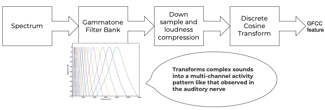
Figure 3:GFCC from audio spectrum.
GFCCs are formed by passing the spectrum through a gammatone filter bank, followed by loudness compression and DCT, as seen in Figure 3. The first (approximately) 22 features are called GFCCs. GFCCs have a number of applications in speech processing, such as speaker identification. GFCC for a sample speech audio can be seen in Figure 4.

Figure 4:GFCC from a sample speech audio.
Temporal features
Temporal features from audio are extracted from the signal information in its time domain representations. Examples include signal energy, entropy, zero crossing rate, etc. Some sample mean temporal features can be seen in Figure 5.

Figure 5:Temporal extractions from a sample speech audio.
Spectral features
Spectral features on the other hand derive information contained in the frequency domain representation of an audio signal. The signal can be converted from time domain to frequency domain using the Fourier transform. Useful features from the signal spectrum include fundamental frequency, spectral entropy, spectral spread, spectral flux, spectral centroid, spectral roll-off, etc. Some sample mean spectral features can be seen in Figure 6.

Figure 6:Spectral features from a sample speech audio.
Chroma features
Chroma features are highly popular for music audio data. In Western music, the term chroma feature or chromagram closely relates to the twelve different pitch classes. Chroma-based features, which are also referred to as “pitch class profiles”, are a powerful tool for analyzing music whose pitches can be meaningfully categorized (often into twelve categories : A, A#, B, C, C#, D, D#, E, F, F#, G, G# ) and whose tuning approximates to the equal-tempered scale Wikipedia contributors, 2022. A prime characteristic of chroma features is that they capture the harmonic and melodic attributes of audio, while being robust to changes in timbre and instrumentation. Some sample mean chroma features can be seen in Figure 7.

Figure 7:Chroma features from a sample speech audio.
Audio data cleaning/de-noising
Often times an audio sample has multiple segments present in the same signal that do not contain anything but silence or a slight degree of background noise compared to the rest of the audio. For most applications, those low activity segments make up the irrelevant information of the signal.
The audio clip shown in Figure 8 is a human saying the word “london” and represents the audio plotted in the time domain, with signal amplitude as y-axis and sample number as x-axis. The areas where the signal looks closer to zero/low in amplitude are areas where speech is absent and represents the pauses the speaker took while saying the word “london”.

Figure 8:Time-series representation of speech for “london”.
Figure 9 shows the spectrogram of the same audio signal. A spectrogram contains time on the x-axis and frequency of the y-axis. A spectrogram is a visual representation of the spectrum of frequencies of a signal as it varies with time. When applied to an audio signal, spectrograms are sometimes called sonographs, voiceprints, or voicegrams. When the data are represented in a 3D plot they may be called waterfalls. As Wikipedia contributors (2021) mentions, spectrograms are used extensively in the fields of music, linguistics, sonar, radar, speech processing, seismology, and others. Spectrograms of audio can be used to identify spoken words phonetically, and to analyze the various calls of animals. A spectrogram can be generated by an optical spectrometer, a bank of band-pass filters, by Fourier transform or by a wavelet transform. A spectrogram is usually depicted as a heat map, i.e., as an image with the intensity shown by varying the color or brightness.

Figure 9:Spectrogram of speech for “london”.
After applying the algorithm for signal alteration to remove irrelevant and low activity audio segments, the resultant audio’s time-series plot looks like Figure 10. The spectrogram looks like Figure 11. It can be seen that the low activity areas are now missing from the audio and the resultant audio contains more activity filled regions. This algorithm removes silences as well as low-activity regions from the audio.

Figure 10:Time-series representation of cleaned speech for “london”.

Figure 11:Spectrogram of cleaned speech for “london”.
These visualizations were produced using pyAudioProcessing and can be produced for any audio signal using the library.
Impact of cleaning on feature formations for a classification task
A spoken location name classification problem was considered for this evaluation. The dataset consisted of 23 samples for training per class and 17 samples for testing per class. The total number of classes is 2 - london and boston. This dataset was manually created and can be found linked in the project readme of pyAudioProcessing. For comparative purposes, the classifier is kept constant at SVM, and the parameter C is chosen based on grid search for each experiment based on best precision, recall and F1 score. Results in Table 4 show the impact of applying the low-activity region removal using pyAudioProcessing prior to training the model using MFCC features.
It can be seen that the accuracies increased when audio samples were cleaned prior to training the model. This is especially useful in cases where silence or low-activity regions in the audio do not contribute to the predictions and act as noise in the signal.
Table 4:Performance comparison on test data between MFCC feature trained model with and without cleaning.
| Features | boston acc | london acc |
|---|---|---|
| mfcc | 0.765 | 0.412 |
| clean+mfcc | 0.823 | 0.471 |
Integrations
pyAudioProcessing integrates with third-party tools such as scikit-learn, matplotlib, and pydub to offer additional functionalities.
Training, classification, and evaluation
The library contains integrations with scikit-learn classifiers for passing audio through feature extraction followed by classification directly using the raw audio samples as input. Training results include computation of cross-validation results along with hyperparameter tuning details.
Audio format conversion
Some applications and integrations work best with .wav data format. pyAudioProcessing integrates with tools that perform format conversion and presents them as a functionality via the library.
Audio visualization
Spectrograms are 2-D images representing sequences of spectra with time along one axis, frequency along the other, and brightness or color representing the strength of a frequency component at each time frame Wyse, 2017. Not only can one see whether there is more or less energy at, for example, 2 Hz vs 10 Hz, but one can also see how energy levels vary over time PNSN, n.d.. Some of the convolutional neural network architectures for images can be applied to audio signals on top of the spectrograms. This is a different route of building audio models by developing spectrograms followed by image processing. Time-series, frequency-domain, and spectrogram (both time and frequency domains) visualizations can be retrieved using pyAudioProcessing and its integrations. See Figure 10 and Figure 9 as examples.
Conclusion
In this paper pyAudioProcessing, an open-source Python library, is presented. The tool implements and integrates a wide range of audio processing functionalities. Using pyAudioProcessing, one can read and visualize audio signals, clean audio signals by removal of irrelevant content, build and extract complex features such as GFCC, MFCC, and other spectrum and cepstrum based features, build classification models, and use pre-built trained baseline models to classify different types of audio. Wrappers along with command-line usage examples are provided in the software’s readme and wiki for giving the user a guide and the flexibility of usage. pyAudioProcessing has been used in active research around audio processing and can be used as the basis for further python-based research efforts.
pyAudioProcessing is updated frequently in order to apply enhancements and new functionalities with recent research efforts of the digital signal processing and machine learning community. Some of the ongoing implementations include additions of cepstral features such as LPCC, integration with deep learning backends, and a variety of spectrogram formations that can be used for image classification-based audio classification tasks.
Copyright © 2022 Singh. This is an open-access article distributed under the terms of the Creative Commons Attribution 3.0 Unported license.
- ADHD
- Attention Deficit Hyperactivity Disorder
- BFCC
- Bark Frequency Cepstral Coefficients
- DCT
- discrete cosine transform
- GFCC
- Gammatone Frequency Cepstral Coefficients
- k-NN
- k-nearest neighbors
- LPC
- Linear Prediction Coefficients
- LPCC
- Linear Prediction Cepstral Coefficients
- MFCC
- Mel Frequency Cepstral Coefficients
- PNCC
- Power Normalized Cepstral Coefficients
- RBF
- radial basis function
- SVM
- support vector machine
- Wikipedia contributors. (2022). Word embedding — Wikipedia, The Free Encyclopedia. https://en.wikipedia.org/w/index.php?title=Word_embedding&oldid=1091348337
- Jyotika Singh. (2021). Social Media Analysis using Natural Language Processing Techniques. In Meghann Agarwal, Chris Calloway, Dillon Niederhut, & David Shupe (Eds.), Proceedings of the 20th Python in Science Conference (pp. 52–58). 10.25080/majora-1b6fd038-009
- Singh, J. (2021). jsingh811/pyAudioProcessing: Audio processing, feature extraction and classification (v1.2.0) [Computer software]. Zenodo. 10.5281/zenodo.5121041
- McFee, B., Raffel, C., Liang, D., Ellis, D. P., McVicar, M., Battenberg, E., & Nieto, O. (2015). librosa: Audio and music signal analysis in python. Proceedings of the 14th Python in Science Conference, 8. 10.5281/zenodo.4792298
- Malek, A. (2020). spafe/spafe: 0.1.2 (0.1.2) [Computer software]. https://github.com/SuperKogito/spafe
- Bogdanov, D., Wack, N., Gómez, E., Gulati, S., Herrera, P., Mayor, O., Roma, G., Salamon, J., Zapata, J., & Serra, X. (2013, November). ESSENTIA: an Audio Analysis Library for Music Information Retrieval. Proceedings - 14th International Society for Music Information Retrieval Conference.
- Giannakopoulos, T. (2015). pyAudioAnalysis: An Open-Source Python Library for Audio Signal Analysis. PloS One, 10(12). 10.1371/journal.pone.0144610
- Auffarth, B. (2020). Artificial Intelligence with Python Cookbook. Packt Publishing.
- Dinger, V. (2021). Master Thesis KI Methodiken für die Verarbeitung akustischer Signale AI Usage for Processing Acoustic Signals [Phdthesis, Kaiserslautern University of Applied Sciences]. 10.13140/RG.2.2.15872.97287
- Balaji, S., Gopannagari, M., Sharma, S., & Rajgopal, P. (2021). Developing a Machine Learning Algorithm to Assess Attention Levels in ADH Students in a Virtual Learning Setting using Audio and Video Processing. International Journal of Recent Technology and Engineering (IJRTE), 10(1). 10.35940/ijrte.A5965.0510121
- PePy. (2022). PePy download statistics. https://pepy.tech/project/pyAudioProcessing
- Chauhan, P. M., & Desai, N. P. (2014). Mel Frequency Cepstral Coefficients (MFCC) based speaker identification in noisy environment using wiener filter. 2014 International Conference on Green Computing Communication and Electrical Engineering (ICGCCEE), 1–5. 10.1109/ICGCCEE.2014.6921394
- Jeevan, M., Dhingra, A., Hanmandlu, M., & Panigrahi, B. (2017). Robust Speaker Verification Using GFCC Based i-Vectors (Vol. 395, pp. 85–91). Springer. 10.1007/978-81-322-3592-7_9
- Tzanetakis, G., Essl, G., & Cook, P. (2001). Automatic Musical Genre Classification Of Audio Signals. The International Society for Music Information Retrieval. http://ismir2001.ismir.net/pdf/tzanetakis.pdf
- Singh, J. (2019). An introduction to audio processing and machine learning using Python. In Opensource article. Opensource. https://opensource.com/article/19/9/audio-processing-machine-learning-python