Performing Object Detection on Drone Orthomosaics with Meta's Segment Anything Model (SAM)
Abstract
Accurate and efficient object detection and spatial localization in remote sensing imagery is a persistent challenge. In the context of precision agriculture, the extensive data annotation required by conventional deep learning models poses additional challenges. This paper presents a fully open source workflow leveraging Meta AI’s Segment Anything Model (SAM) for zero-shot segmentation, enabling scalable object detection and spatial localization in high-resolution drone orthomosaics without the need for annotated image datasets. Model training and/or fine-tuning is rendered unnecessary in our precision agriculture-focused use case. The presented end-to-end workflow takes high-resolution images and quality control (QC) check points as inputs, automatically generates masks corresponding to the objects of interest (empty plant pots, in our given context), and outputs their spatial locations in real-world coordinates. Detection accuracy (required in the given context to be within 3 cm) is then quantitatively evaluated using the ground truth QC check points and benchmarked against object detection output generated using commercially available software. Results demonstrate that the open source workflow achieves superior spatial accuracy — producing output 20% more spatially accurate, with 400% greater IoU — while providing a scalable way to perform spatial localization on high-resolution aerial imagery (with ground sampling distance, or GSD, < 30 cm).
2Introduction
Image segmentation is a critical task in geospatial analysis, enabling the identification and extraction of relevant features from high resolution remote sensing imagery Wu & Osco, 2023. However, extracting actionable information (i.e., object detection and spatial localization) can be constrained by the need for large, labeled datasets to train deep learning models in order to then perform inference and (hopefully) produce the desired output. This bottleneck is particularly acute in agricultural domains, where variability in conditions and object types complicates manual annotation Osco et al., 2023.
Recent advances in foundation models, such as Meta AI’s Segment Anything Model (SAM), offer a promising path forward. SAM is designed for promptable “zero-shot” segmentation. “Prompt engineering”, in this context, involves using points and bounding boxes to focus the model’s efforts on more efficiently generating masks corresponding to objects of interest Mayladan et al., 2024. Providing these prompts allows accurate masks to be generated for novel objects (ones not included in SAM’s training corpus), without domain-specific training. Masks can also be generated automatically with no such prompting. SAM’s automatic mask generator will effectively “detect” everything using open source model checkpoints and generate masks for each object in a provided image Kirillov et al., 2023.
While SAM’s ability to generalize is impressive Kirillov et al., 2023Osco et al., 2023, its performance on remote sensing imagery and fine-grained features requires careful workflow integration and evaluation Wu & Osco, 2023. This paper describes a comprehensive, open source workflow for object detection and spatial localization in high-resolution remote sensing imagery, built around SAM and widely used geospatial Python libraries GDAL/OGR contributors, 2025Gillies et al., 2025Jordahl et al., 2020Gillies & others, 2013. The complete process is delineated, from data loading and preprocessing to mask generation, post-processing, and quantitative accuracy assessment, culminating in a rigorous comparison against the results produced using the proprietary software (see code). Precision, accuracy, F1 score, mean deviation (in cm), and Intersection-over-Union (IoU) are calculated in order to quantify the relative quality of the output produced using each workflow[1].
3Motivation
Precision agriculture relies on accurate object detection for tasks such as plant counting, health monitoring, and the automated control of heavy equipment. Traditional deep learning approaches can become hindered by the cost and effort of generating carefully annotated data, limiting scalability and accessibility. Proprietary solutions, while effective, can be expensive and opaque, impeding reproducibility and customization.

Figure 1:The derived centroids of the objects detected in drone orthomosaics are used to automate this nursery trimmer.
SAM’s zero-shot segmentation capability directly addresses the data annotation bottleneck, enabling rapid deployment in novel contexts. By developing an open source workflow around SAM, an end-to-end pipeline is created which allows for the quantitative evaluation of spatial accuracy with respect to objects detected in high-resolution aerial imagery. This modular workflow can also be repurposed as an automated data annotation pipeline for downstream model training/fine-tuning, if required[2].
4Approach
Our approach integrates SAM’s segmentation strengths with traditional geospatial data processing techniques, which lends itself to our precision agriculture use case. The workflow, like any other, can be thought of as a sequence of steps (visualized above and described below), each with their own sets of substeps:
Data Ingestion: Loading GeoTIFF orthomosaics and QC point CSVs, extracting spatial bounds and coordinate reference systems (CRS) using Rasterio or GDAL.
Preprocessing: Filtering QC points to those within image bounds, standardizing coordinate columns, and saving filtered data for downstream analysis.
Mask Generation: Tiling large images for efficient processing, running SAM’s automatic mask generator (ViT-H variant) on each tile, and filtering masks by confidence.
Post-Processing: Converting masks to polygons, filtering by area and compactness, merging overlapping geometry, and extracting centroids.
Accuracy Evaluation: Calculating point-to-centroid deviations (in centimeters) between detected objects and QC points, compiling results, and generating visual and tabular reports.
Benchmarking: Quantitatively comparing SAM-based results against the evaluated output using identical evaluation metrics (precision, recall, IoU, etc.; see Appendix for details).
It should be noted that there are no model training or fine-tuning steps included in our workflow, as we are using a foundation model to generate masks. This is analogous to using ChatGPT to generate text, which does not require users to train or fine-tune the underlying foundation model in order to do so.
This approach is carried out entirely using open source Python libraries, ensuring transparency and extensibility.
5Methodology
5.1Data and Environment
Imagery: High-resolution GeoTIFF orthomosaic.
Image size: 18,200 x 55,708; 1,013,885,600 pixels
Total area: 545,243 sq ft; 12.5 acres
GSD: 0.71 cm
Ground Truth: QC points in CSV format, containing spatial coordinates and unique identifiers.
Coordinate Reference System (CRS) Transformations: All spatial operations are performed using the NAD83 CRS (EPSG:6859), with reprojection to the WGS84 CRS (EPSG:4326) for downstream reporting and nursery trimmer automation.
Dependencies[3]:
GeoPandas Jordahl et al., 2020
Matplotlib Hunter, 2007
NumPy Harris et al., 2020
OpenCV Bradski, 2000
OpenPyXL Gazoni & Clark, 2024
Pillow Clark, 2015
Rasterio Gillies & others, 2013
Segment Anything[4] Kirillov et al., 2023
Shapely Gillies et al., 2025
Torch Paszke et al., 2019
5.2Workflow
5.2.1Data Ingestion and Preprocessing
5.2.2Mask Generation
5.2.3Post-Processing
5.2.4Accuracy Evaluation
See Appendix for accuracy evaluation methodology details.
5.2.5Benchmarking
See code for benchmarking methodology details.
6Results
6.1Proprietary Workflow

Figure 2:19 false positives (FP) and hundreds of sliver polygons were observed in the output produced using the proprietary software.
The bounding boxes that were output using this workflow (against which we are benchmarking ours) can be viewed as a layer overlain onto the GeoTIFF orthomosaic using GIS software[5]. What was of particular use to us is the fact that zero false negatives (FN) were observed in the output, though 19 false positives (FP) were. This empirical knowledge equips us with something not usually possessed in use cases such as this: the number of true positives (TP), which allows us to leverage such metrics as precision, recall, and the harmonic mean of the two, F1 score, to perform a rigorous comparison against our open source workflow (see code).
6.2Open Source Workflow

Figure 3:18 FP were observed in the output produced using the open source workflow.
Merging the overlapping geometry and filtering out the empirically observed FP allowed for us to ascertain exactly how many TP (18,736) there are in the benchmark output and derive how many FP (18) and FN (65) there are in our workflow output, which enabled us to conduct our performance comparison.
Table 1:Performance Comparison
| Workflow | Detection Quality Metrics | Localization Accuracy Metrics | |||
|---|---|---|---|---|---|
| Precision | Recall | F1 Score | Mean Deviation (cm) | IoU | |
| Proprietary | 0.9990 | 1.0000 | 0.9995 | 1.39 | 0.18 |
| Open Source | 0.9990 | 0.9956 | 0.9973 | 1.20 | 0.74 |
It can be observed that empty plant pots tend to be ~64 pixels (px) wide and tall; with QC points corresponding to actual pot centroids, we were able to create 64-by-64px boxes to facilitate our IoU calculations (see code). These calculations further allow us to assess the relative alignment between the detection output geometry and our “ground truth” geometry.
This work makes it easy to identify down to the individual QC point ID level which detection centroids deviate from said point by more than 3 cm, which is the tolerance specified by our client. In aggregate, we were able to gain a quantified sense of the mean deviation (in cm) of the output produced by each workflow. However, visual inspection revealed that some detection geometry was flagged as having out-of-tolerance centroids when the QC points were themselves off-center. This is to say that some detections from both workflows were flagged as being out-of-tolerance when they observably were not.

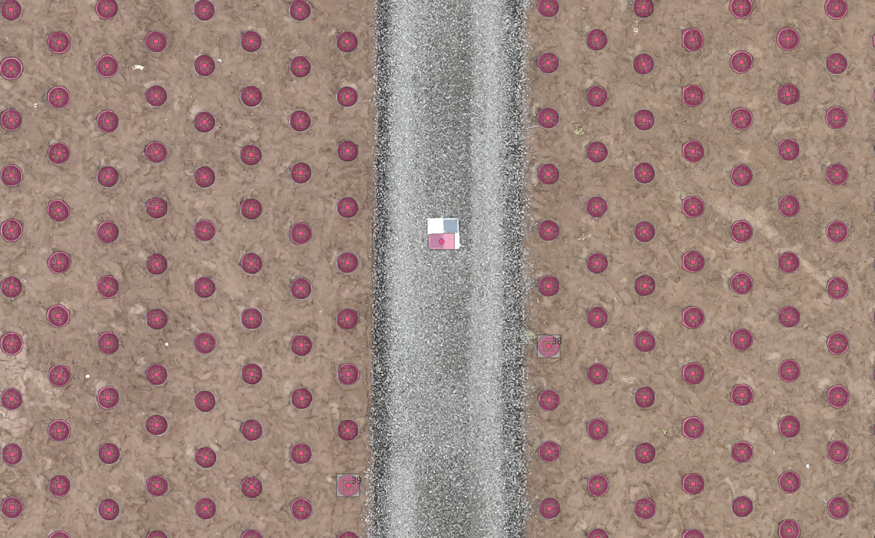
Figure 4:Visual inspection of the detected centroids relative to QC point 91 reveal that the QC point is off-center.
Visual inspection also reveals that our detections (the pink circle) and those produced using the commercial software (the beige square) have greater overall coverage with respect to the QC geometry (the grey square). This provides intuition as to why the IoU calculations revealed a 400% increase in coverage with respect to the geometry produced using SAM’s automatic mask generator, zero-shot.
7Discussion
7.1Key Findings
The open-source workflow powered by Meta AI’s Segment Anything Model (SAM) outperformed a commercial alternative in object detection and spatial localization on high-resolution drone imagery. It achieved 20% higher spatial accuracy (1.20 cm vs. 1.39 cm deviation) and a 400% higher Intersection-over-Union (IoU) (0.74 vs. 0.18), indicating stronger alignment between the detections and the actual object boundaries. Both methods had near-perfect precision, but the open-source approach showed slightly lower recall due to 65 false negatives. It should be noted, however, that these FN were a direct result of the filtering substep in our workflow, which excludes detections outside of the provided geometry area and compactness thresholds; see code.
Nevertheless, its overall performance supports its suitability for precision agriculture and downstream automation.
7.2Precision Agriculture Challenges
Our work began with an eye toward tackling a major challenge in agricultural remote sensing: the need for extensive manual annotation. SAM’s zero-shot segmentation enables accurate object detection without domain-specific training, making it scalable and adaptable for new use cases with minimal setup.
7.3Benefits of Open Source
Built entirely on open source geospatial tools, our open source workflow offers transparency, reproducibility, and flexibility. It can be tailored to suit various tasks, even automating annotation for model training, thereby supporting broader adoption with respect to high-resolution remote sensing imagery, in general.
7.4Practical Impact
Meeting professional-grade tolerance requirements (e.g., < 3 cm) enables real-world applications, such as automating heavy equipment, based on precise object localization. This demonstrates how automated workflows can reduce manual labor and support more efficient agricultural practices.
7.5Limitations and Future Work
Our approach to tiling (“chipping”) high-resolution orthomosaics, processing 588 individual 1280-by-1280px tiles at an average pace of 11 seconds per tile, required a total processing time of ~110 minutes running on a Colab single T4 GPU instance. It is important to note that an overlap of 25% (320px) between tiles during processing was required to ensure that geometry was not produced containing “holes” or malformations; merging overlapping polygons after filtering (based on area and compactness calculations, in this case) helped us ensure the overall quality of the geometric output.
Future work will be centered on building an open source CLI and Python package[6], which will allow users to pass orthomosaics as inputs and get geometry meeting desired spatial charactersitics as an output.
8Conclusion
We present a robust, open source workflow for object detection and spatial localization in high-resolution drone orthomosaics, leveraging SAM’s zero-shot segmentation capabilities. Our quantitative evaluation demonstrates improved accuracy over a commercially available software solution, underscoring the potential of foundation models and open source tools to advance scalable, cost-effective feature extraction. This work provides a template for further research and deployment in diverse contexts.
To our knowledge, this is the first comparative evaluation of an open source segmentation model against commercial software in a context requiring high (< 3 cm) spatial accuracy. Our results demonstrate that the workflow not only matches but in some cases exceeds performance metrics with respect to the evaluated output.
9Conflicts of Interest
The author declares no conflicts of interest.
10AI Usage Disclosure
AI tools (ChatGPT, Perplexity, and NotebookLM) were used:
in writing portions of the workflow integration code,
to generate Matplotlib subplots, process flow diagrams, pseudocode, L A T E X, etc.
for proofreading and light revision to reduce potential publication errors.
11Code
Data and code required to replicate our approach can be found using the links below:


12Appendix
12.1Accuracy Evaluation Methodology
The evaluation focuses on two primary categories of metrics: localization accuracy and detection quality; the employed methodology relies on the following data:
Ground Truth Quality Control (QC) Points (), defined as a set of known spatial coordinates, , where each represents the centroid (in real-world coordinates) of our object of interest (empty plant pots), serving as the ground truth for spatial localization.
Detected Object Centroids () are used, which are a set of centroids, , where each is the centroid extracted from a polygon representing an object detected by the workflow.
Detected Object Polygons () are included, representing a set of polygons, where each is a polygon generated from a SAM-produced mask after post-processing.
Ground Truth Polygons () the calculation of Intersection over Union (IoU) implies the existence of a corresponding set of ground truth polygons, , where each delineates the extent of the object associated with ground truth point . This allows for the quantification of the spatial alignment between the detection bounding boxes and those associated with the QC points, in aggregate. The provided code details how we created this geometry and performed the calculations.
We gratefully acknowledge the contributions of the open source community — thank you to the giants on whose shoulders we stand.
This work was funded by FiOR Innovations and Woodburn Nursery & Azaleas. We deeply appreciate their support and partnership.
A special thanks to Paniz Herrera, MBA, MSIST, Ryan Marinelli, PhD Fellow at the University of Oslo, and Danny Clifford for their help proofreading.
Copyright © 2025 McCarty. This is an open-access article distributed under the terms of the Creative Commons Attribution 4.0 International license, which enables reusers to distribute, remix, adapt, and build upon the material in any medium or format, so long as attribution is given to the creator.
See this Colab notebook for details.
See requirements.txt for version details.
Inference was accelerated using
CUDA 12(cuDF 25.2.1) on aT4GPU within our Colab notebook environment.We used open source QGIS QGIS Development Team, 2021 as our selected data viewer.
We have since open-sourced the
orthomaskerPython package and CLI; work on a GUI is currently underway.
- CRS
- coordinate reference system
- FN
- false negatives
- FP
- false positives
- GSD
- ground sampling distance
- IoU
- Intersection-over-Union
- QC
- quality control
- SAM
- Segment Anything Model
- TP
- true positives
- Wu, Q., & Osco, L. P. (2023). samgeo: A Python package for segmenting geospatial data with the Segment Anything Model (SAM). Journal of Open Source Software, 8(89), 5663. https://doi.org/10.21105/joss.05663
- Osco, L. P., Wu, Q., de Lemos, E. L., Gonçalves, W. N., Ramos, A. P. M., Li, J., & Junior, J. M. (2023). The Segment Anything Model (SAM) for Remote Sensing Applications: From Zero to One Shot. https://doi.org/10.48550/arXiv.2306.16623
- Mayladan, A., Nasrallah, H., Moughnieh, H., Shukor, M., & Ghandour, A. J. (2024). Zero-Shot Refinement of Buildings’ Segmentation Models using SAM. https://doi.org/10.48550/arXiv.2310.01845
- Kirillov, A., Mintun, E., Ravi, N., Mao, H., Rolland, C., Gustafson, L., Xiao, T., Whitehead, S., Berg, A. C., Lo, W.-Y., Dollár, P., & Girshick, R. (2023). Segment Anything. https://doi.org/10.48550/arXiv.2304.02643
- GDAL/OGR contributors. (2025). GDAL/OGR Geospatial Data Abstraction software Library. Open Source Geospatial Foundation. 10.5281/zenodo.5884351
- Gillies, S., van der Wel, C., Van den Bossche, J., Taves, M. W., Arnott, J., Ward, B. C., & others. (2025). Shapely (Version 2.1.1). 10.5281/zenodo.5597138
- Jordahl, K., den Bossche, J. V., Fleischmann, M., Wasserman, J., McBride, J., Gerard, J., Tratner, J., Perry, M., Badaracco, A. G., Farmer, C., Hjelle, G. A., Snow, A. D., Cochran, M., Gillies, S., Culbertson, L., Bartos, M., Eubank, N., maxalbert, Bilogur, A., … Leblanc, F. (2020). geopandas/geopandas: v0.8.1 (v0.8.1). Zenodo. 10.5281/zenodo.3946761
- Gillies, S., & others. (2013–). Rasterio: geospatial raster I/O for Python programmers. Mapbox. https://github.com/rasterio/rasterio
- Hunter, J. D. (2007). Matplotlib: A 2D graphics environment. Computing in Science & Engineering, 9(3), 90–95. https://doi.org/10.1109/MCSE.2007.55
- Harris, C. R., Millman, K. J., van der Walt, S. J., Gommers, R., Virtanen, P., Cournapeau, D., Wieser, E., Taylor, J., Berg, S., Smith, N. J., Kern, R., Picus, M., Hoyer, S., van Kerkwijk, M. H., Brett, M., Haldane, A., del Río, J. F., Wiebe, M., Peterson, P., … Oliphant, T. E. (2020). Array programming with NumPy. Nature, 585(7825), 357–362. https://doi.org/10.1038/s41586-020-2649-2
- Bradski, G. (2000). The OpenCV Library. Dr. Dobb’s Journal of Software Tools.
- Gazoni, E., & Clark, C. (2024). OpenPyXL: A Python library to read/write Excel 2010 xlsx/xlsm/xltx/xltm files. Python Package. https://openpyxl.readthedocs.io
- The Pandas Development Team. (2020). pandas-dev/pandas: Pandas (latest). Zenodo. 10.5281/zenodo.3509134
- McKinney, W. (2010). Data Structures for Statistical Computing in Python. In Stéfan van der Walt & Jarrod Millman (Eds.), Proceedings of the 9th Python in Science Conference (pp. 56–61). https://doi.org/10.25080/Majora-92bf1922-00a
- Clark, A. (2015). Pillow (PIL Fork) Documentation. readthedocs. https://buildmedia.readthedocs.org/media/pdf/pillow/latest/pillow.pdf