
Imprecise uncertainty management with uncertain numbers to facilitate trustworthy computations
Abstract
Scientific computations of complex systems are surrounded by various forms of uncertainty, requiring appropriate treatment to maximise the credibility of computations. Empirical information for characterisation is often scarce, vague, conflicting and imprecise, requiring expressive uncertainty structures for trustworthy representation, aggregation and propagation. Current practices may present two undesired extremes in terms of uncertainty management, with one endpoint being the total ignorance of uncertainty, whereas the other suggesting overconfidence through the introduction of assumptions unjustified by empirical information. In response to these challenges, this paper demonstrates the framework of uncertain number, a unified construct for expressive uncertainty representation at different imprecision. This framework, embedded in the library pyuncertainnumber, allows for a closed computation ecosystem whereby trustworthy computations can be conducted intrusively or non-intrusively, hence accomplishing faithful management of uncertainty throughout the computational pipeline. This paper presents an overview of the main capabilities and features of pyuncertainnumber.
1Introduction
Large-scale scientific computing applications for complex physical and engineered systems are often approximate and uncertain, notably due to limited knowledge of the physical processes, approximate representation of the model, and sparse experimental data for calibration, etc Roy & Oberkampf, 2011Oberkampf et al., 2004Smith, 2024. Besides, engineered systems are often required to operate safely and robustly under varying environments or uncertain operational conditions, requiring uncertainty to be comprehensively considered in order to maximise the credibility of predictions, designs and decisions Gray et al., 2022.
It is vital to know what you do not know in terms of trustworthy modelling and predictions, suggesting that all models are wrong but some are useful on the condition of knowing their assumptions and applicability, hence building the credibility of the computational results. It is often a challenge, in modelling complex physical phenomena, to construct mathematical models in a quantitative manner, on one hand, without ignoring significant information and, on the other hand, without introducing unwarranted assumptions Beer et al., 2013Patelli et al., 2017. The bottleneck is usually the limited information in terms of both knowledge and experimental data.
The increasing awareness of the differentiation of aleatory and epistemic uncertainty arises the need for more expressive mathematical frameworks to reason with various forms of uncertainty Ferson & Hajagos, 2004Ferson & Ginzburg, 1996. Imprecise uncertainty frameworks Destercke et al., 2008, such as evidence theory, random set, possibility distributions, credal set, capacities are proposed to reflect the situations when information is scarce, vague, conflicting or imprecise whereby precise distribution are hard to be defined. Given the available information, there exist two untenable extreme (exclusive) endpoints that prescribe an interval of trustworthiness. The lack of uncertainty quantification presented in many deterministic numerical simulations constitutes the lower bound, whereas the overconfidence of the computation, through introduction of unwarranted assumptions about uncertainties not faithful to the state of knowledge, as the upper bound.
We aim at a faithful management of uncertainty throughout the computational pipeline using uncertain number, a unified construct for uncertainty characterisation at different imprecision.
This paper demonstrates the framework of uncertain number which allows for a closed computation ecosystem whereby trustworthy computations can be conducted in a rigorous manner.
This paper presents an overview of the main capabilities of the library pyuncertainnumber[1]. To facilitate clearer illustration and reproducibility of the workflow, essential code snippets are included in the main text, while a comprehensive tutorial is available in the Supporting Documents section.
2Expressive power of uncertain number
When characterising input parameters to a simulation model, while probability distribution has long been used to reflect uncertainty (variability[2]), there is still uncertainty (incertitude[3]) about the distribution shape and interdependencies. Empirical information varies in quality and nature, which may be quantitative, qualitative and even linguistically vague. Multiple sources or elicitation could vary in credibility and even be conflicting. Empirical data, if any, may be scarce or imprecise due to the inaccuracy of experimental measurements, or prohibitive cost of collecting data. It is therefore challenging to formulate suitable uncertainty models given partial information without introducing unwarranted assumptions. To this end, more expressive mathematical constructs are needed.
Uncertain number stands for a generalised representation that unifies several uncertainty constructs including intervals, probability distributions, probability boxes (p-boxes) and Dempster-Shafer structures (DSS), plus real numbers.
These constructs are closely related to each other: an interval indicates a value imprecisely known within a range where no assumptions of likelihood about the enclosed values are made; P-boxes can be considered as interval bounds on cumulative distributions and a DSS can be deemed as a discrete distribution with interval quantiles.
Parametric p-boxes are probability distributions whose parameters and samples are intervals, and an interval () can be identified as a p-box whose bounds are unit step functions denoted by ; a p-box can be discretised into a DSS with pairs of intervals (focal elements) and probability masses , and conversely a DSS can be stacked with a list of intervals. Importantly, all of these constructs are special cases of free p-boxes which effectively represents a set of distributions.
Figure 1 visually illustrates the notion of an uncertain number, which is underpinned by a probability bounding approach Williamson & Downs, 1990Ferson et al., 2003Gray et al., 2022 that allows for a faithful representation of the state of empirical information. For example, it can be characterised as a real number (a degenerate of an interval) when there is no uncertainty, a precise distribution (a degenerate of a p-box) when there is abundant data, and a set of distributions (e.g. a p-box) when there is partial information.
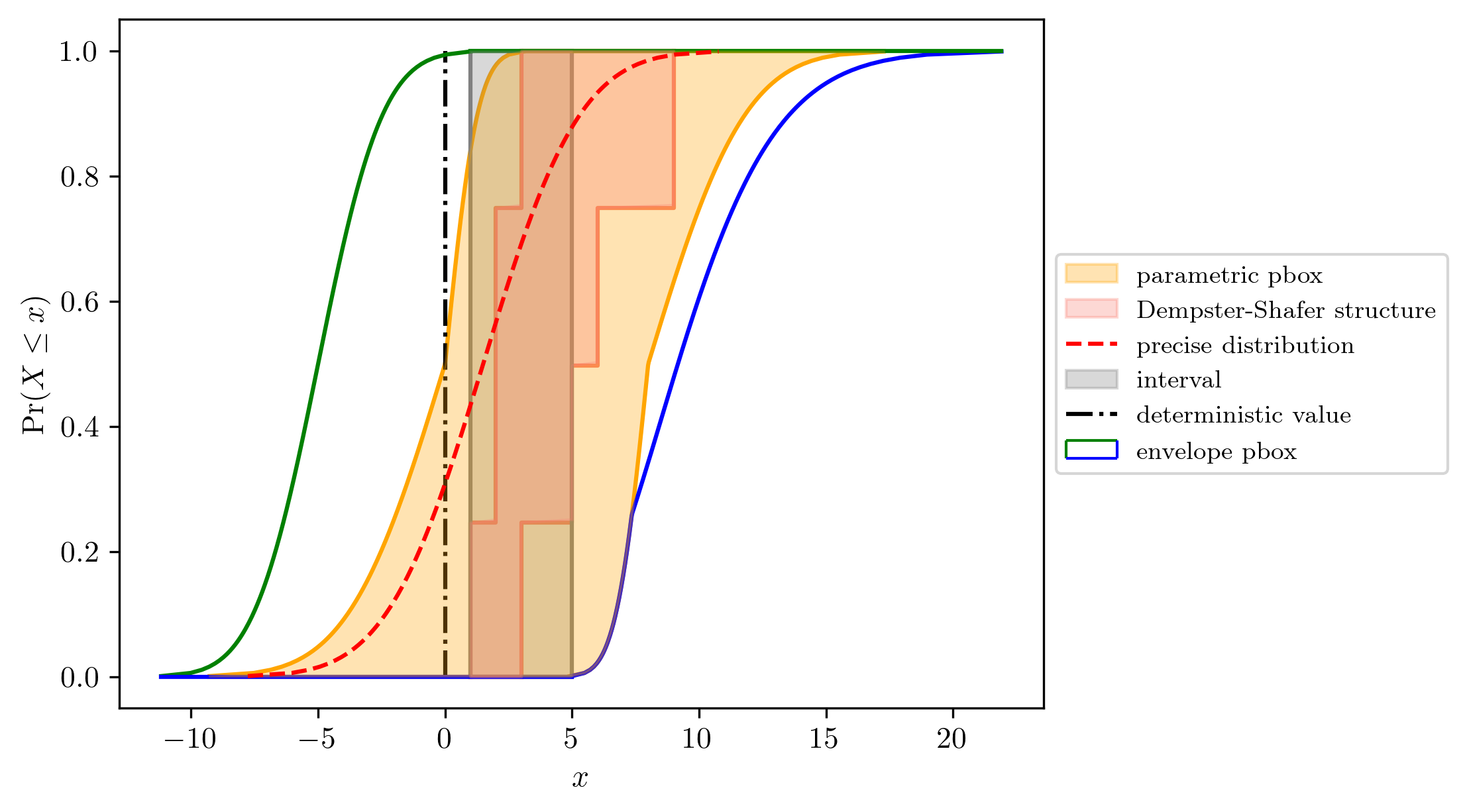
Figure 1:Uncertain number refers to a generalised representation that unifies several constructs including intervals, probability distributions, probability boxes (p-boxes) and Dempster-Shafer structures, plus real numbers.
2.1A probability bounding approach on information constraints
Often there is little empirical information pertaining some parameters of a mathematical model. A faithful characterisation entails that all of the available statistical information should be utilised but without introducing any extra assumptions beyond what are empirically justified.
The bounding approach presents as a natural reflection of the state of epistemic uncertainty, which tightens the bounds with extra empirical information. As shown in Figure 2, the level of information specifies constraints to accordingly construct the uncertain number, which starts as little as a coarse estimated range, to moment information, further to the knowledge of shape such that uncertainties are pinched to a precise distribution. These bounds are best-possible[4] in the sense that they could not be any tighter without excluding CDF satisfying the specified constraints, or without additional information Ferson & Hajagos, 2004.
Conveniently, pyuncertainnumber provides a bespoke constructor to facilitate the faithful characterisation of uncertain quantities based on known information, which includes limits on quantiles, information about summary statistics such as mean, mode or variance, and qualitative information about distribution shape, such as whether it is symmetric or unimodal.
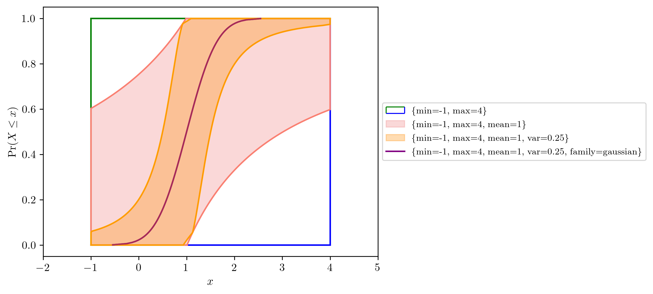
Figure 2:Illustration of the idea of level of information specified as constraints
import pyuncertainnumber as pun

# specify available empirical information as constraints
pun.known_constraints(minimum=0, maximum=2., mean=1, var=0.25)2.2Aggregation of uncertainty
One of the controversial subject in uncertainty analysis is the aggregation of multiple (imperfect) sources of information, evidence, or expert elicitations. Information varies in quality and could be conflicting. Experts may have different degrees of subjectivity and different representations for the uncertain quantity, leading to epistemic uncertainty in the various educated estimates.
Uncertain number presents one advantage that it provides a unified structure to enclose the aggregation operation on a set of expert elicitations, whatever the forms they may be, whether a distribution or an interval.
Figure 3 shows an example of the elicitation from a couple of experts with their credibility shown as probability masses. This explains further the provenance of the constructs in Figure 1.
pyuncertainnumber supports several aggregation rules (e.g. envelope, mixture, and intersection, etc) enabling diverse level of information to be pooled stochastically or conservatively.

Figure 3:Uncertainty aggregation: (a) expert knowledge expressed as intervals coupled with their credibility; (b) the same uncertain number in Figure 1 of which the DSS is composed by the aggregation in (a), and the circumscribed p-box is composed by the envelope in (c); (c) expert elicitation as precise distributions whereby an envelope operation is taken
from pyuncertainnumber import stochastic_mixture, envelope

""" note aggregation operations apply to all constructs of uncertain numbers """

# mixture aggregation of interval elicition into a Dempster-Shafer structure
a = pun.I(1, 5)  # b, c, d ...
mix = stochastic_mixture(a, b, c, d, masses=[0.25, 0.25, 0.25, 0.25])

# envelope aggregation of distributional eclicitation into a p-box
a = pun.D('gaussian', (-5, 2))  # b, c, d ...
env = envelope(a, b, c, d)2.3Measurement imprecision
Empirical data rarely come in perfect forms, especially for in situ measurements. Practical computations frequently deal with poor measurements with different imprecision, possibly arising in recording, transmission, communication or manipulation, etc Ferson et al., 2007. Intervals turn out to be natural constructs for representing incertitude in imprecise measurements, manifested either in a direct interval or a plus-or-minus form Angelis, 2022. When interval-valued measurements are present in a data set, a single probability distribution is inadequate to characterise the epistemic uncertainty. Rather, the bounding strategy applies whereby classical inference methods are extended to both characterise the sampling uncertainty and also data imprecision. For example, as shown in Figure 4a, a set of maximum likelihood estimates are yielded for a single datum where indicates the parameter of exponential distribution. Collectively, the dataset leads to an interval bound of the fitted exponential distribution shown in the shaded area in Figure 4b, along with the true data generating mechanism (DGM) in red dotted curve and the empirical CDF in gray dotted curve. Further, as a nonparametric comparison, the Kolmogorov Smirnov confidence bands is also extended Tretiak & Ferson, 2023, as shown in blue dashes below. These are both rigorous uncertain numbers that enclose the true yet unknown data generating distribution.
where and represent the empirical CDF on endpoints of the imprecise dataset, and denotes the Smirnov critical value at significance level .
![Characterisation of imprecise measurements. (a) fitting an exponential distribution to an interval datum by maximum likelihood estimation; (b) Parametric and nonparamettric characterisation of the whole imprecise data set \{ x_{i}\} which includes 15 data points i.i.d (independent and identically distributed) sampled from an exponential distribution (i.e. \text{Exp}(0.4)) contaminated by a margin of error \Delta=1.4. That is, x_{i} = [\underline{x}_i, \overline{x}_i] = [m_{i} - \Delta, m_{i} + \Delta] where m_i \sim \text{Exp}(0.4).](https://pub.curvenote.com/0199eb8c-c4ed-7079-8df8-bc8fe638155d/public/imprecise_measuremen-b06c2bf87ecc1098cf186096cefcac9b.png)
Figure 4:Characterisation of imprecise measurements. (a) fitting an exponential distribution to an interval datum by maximum likelihood estimation; (b) Parametric and nonparamettric characterisation of the whole imprecise data set which includes 15 data points i.i.d (independent and identically distributed) sampled from an exponential distribution (i.e. ) contaminated by a margin of error . That is, where .
import scipy.stats as sps
from pyuncertainnumber import pba

# synthetic generation of the imprecise data
precise_sample = sps.expon(scale=1/0.4).rvs(15)
imprecise_data = pba.I(lo = precise_sample - 1.4, hi=precise_sample + 1.4)

# parametric distributional estimator using method of matching moments
pun.fit('mom', family='exponential', data=imprecise_data)

# nonparametric estimator using Kolmogorov Smirnov confidence bands at 95% confidence level
pun.KS_bounds(imprecise_data, alpha=0.025, display=True)2.4Linguistic numerical hedges for uncertainty interpretation
Minimally, qualitative linguistic description may be used to express the estimates over numerical input values. Those are called numerical hedges, which may include colloquial words such as “about”, “around”, “almost” etc. Ferson et al., 2015.
With the focus on NLP in many deep learning applications in recent years, the interpretation of hedged words and their quantitative implication of uncertainty is vital for downstream safety-related applications.
pyuncertainnumber provides support to interpret these hedges in an effort to build a consistent basis for consistent uncertainty elicitation and communication in situations where empirical information is almost minimal. Importantly, real numbers such as “7” or “7.0” can also be interpreted as an interval based on significant digits Ferson et al., 2015, potentially leading to a complete system of rigorous numerical numbers.
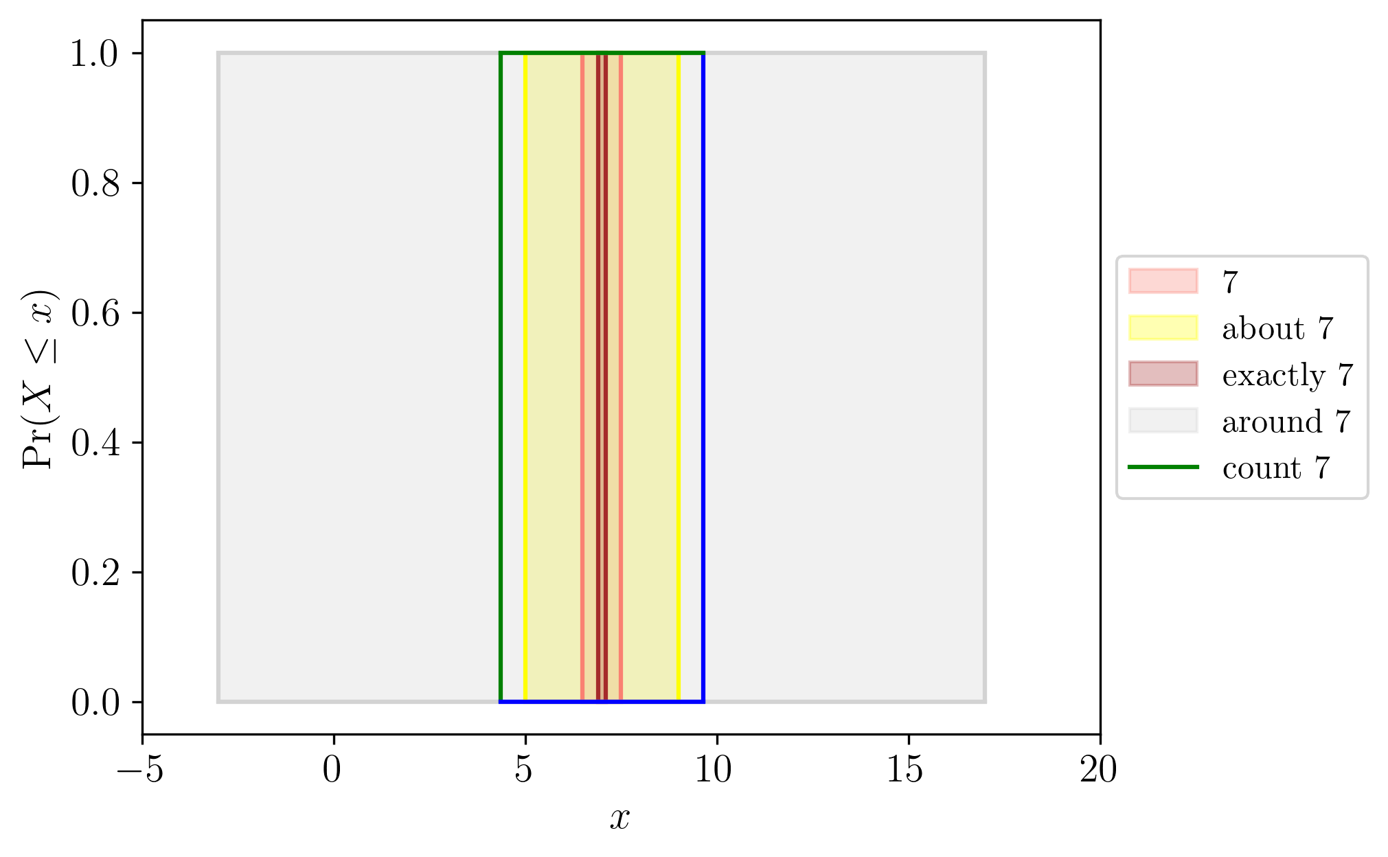
Figure 5:Illustration of numerical hedges.
pun.hedge_interpret('about 7') # similar usage for other hedges, such as '7.0'2.5Dependency structure: fully specified, partially known or unknown
Neglecting the incertitude about the dependency structure and assuming independence anyway constitutes a methodological bad practice. Maybe the most notable example of misuse of dependency structure is the 2008 financial crisis Donnelly & Embrechts, 2010.
Similar as the bounding approach applies onto marginal distributions in the face of various levels of information, the inter-variable dependency information can also be known, partially known or unknown within the probability bounding framework. Collectively, it manifests the imprecise specification of a joint distribution. As an example, Figure 6 illustrates the interval bounds of a joint CDF of a bivariate p-box. In this case, sampling operations will produce bivariate interval constructs, shown as the rectangles at the bottom of Figure 6. These constructs can all be consistently represented as uncertain numbers. Additional details regarding the imprecise dependency specification will be discussed in Section 3.1.
![A bivariate p-box with marginals X \sim \mathcal{B}([4, 8], 3) and Y \sim \mathcal{N}([0,2], 2), and Gaussian copula parameterised by \rho_{XY} = -0.8. The upper of the plot displays the joint CDF with upper and lower surface and the bottom shows the sampled deviates which are bivariate intervals](https://pub.curvenote.com/0199eb8c-c4ed-7079-8df8-bc8fe638155d/public/bivariate_pbox-539bbebd3908344dc68f15bb5df0c0a4.png)
Figure 6:A bivariate p-box with marginals and , and Gaussian copula parameterised by . The upper of the plot displays the joint CDF with upper and lower surface and the bottom shows the sampled deviates which are bivariate intervals
3Non-deterministic computations and uncertainty propagation
Scientific computations are desired to be rigorous and best-possible when subject to uncertainties.
3.1Probability bounds analysis
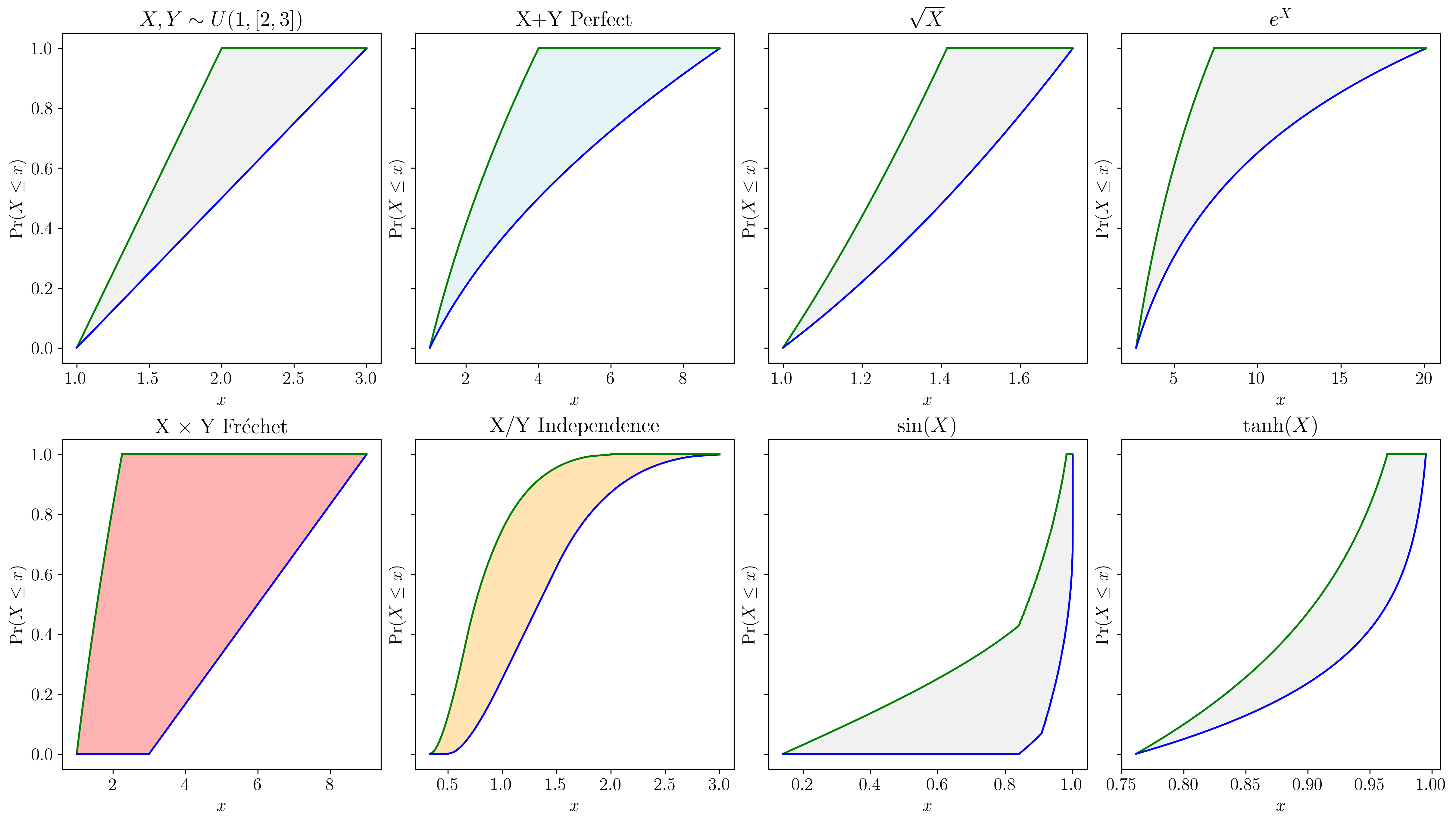
Figure 7:Illustration of p-box arithmetic under various dependency structure. The left four show different dependency structures in colors with different binary operations, the right four show differnt unary operations.
Probability bounds anlaysis (PBA) combines both interval analysis and probability theory, allowing rigorous bounds of (arithmetic) functions of random variables to be computed even with partial information Ferson et al., 2003Ferson & Hajagos, 2004Gray et al., 2022. Intuitively, as interval arithmetic enables rigorous calculation for sets of real numbers, PBA accomplish the same for sets of distributions. P-box arithmetic is built upon generalised probability convolutions, which through further extensions cover a wide spectrum of arithmetic operations: unary transformations, binary operations between p-boxes or Dempster-Shafer structures, and general functions composed of a series of base operations. It also covers a wide spectrum of dependency structures which could be fully known (specified copula ), partially known (lower bound copula ), or even unknown ( bounds Oberkampf et al., 2004).
Importantly, we provide a unified interface and implementation through pyuncertainnumber, enabling rigorous calculations regardless of the representation of the uncertain variables or their dependency structure.
This interface has abstracted out much of the arcane details in terms of conversion, discretisation, condensation, and stacking such that analysts can benefit the consistency and focus more on the effects the calculations.
Notably, the bounds provides a trustworthy default when no dependency information is known, in that the resulting bounds rigorously enclose the result no matter what correlation or nonlinear dependency may exist between these variables. This faithfully translates the situation of unknown into making no assumption at all, as opposed of an unjustified independence assumption. Equation (2) gives the expression Oberkampf et al., 2004 for the addition of uncertain numbers and multiplication and division have similar forms, where denotes the interval bounds of CDF of the composing uncertain number.
Figure 7 displays several common arithmetic examples.
These arithmetic operations can be performed in the same signature in pyuncertainnumber as real number arithmetics in Python via operator overloading. are employed as default except the dependency can be otherwise justified.
Importantly, now these calculations yield regirous results that are guaranteed to enclose all possible distributions of the output variable so long as the input uncertain number were all sure to enclose their respective distributions.
3.2Non-deterministic propagation
Scientific computing typically involves a mathematical model, for example a coupled system of nonlinear partial differential equations, to simulate the behaviour of natural or engineered systems. Many such applications involve high-fidelity numerical solutions as a complicated black-box model (e.g. CFD) in a non-intrusive setting.
For a comprehensive uncertainty analysis, all uncertainty sources (e.g. model inputs, initial or boundary conditions, model form assumptions, numerical approximation, and model extrapolation) should be appropriately characterised and and have their contributions to the total uncertainty of the system response quantity of interest (QoI) elucidated, such that efficient uncertainty reduction or management can be conducted by decision makers. A notable example that embodies the idea of such uncertainty framework is the NASA UQ challenge Crespo & Kenny, 2021.
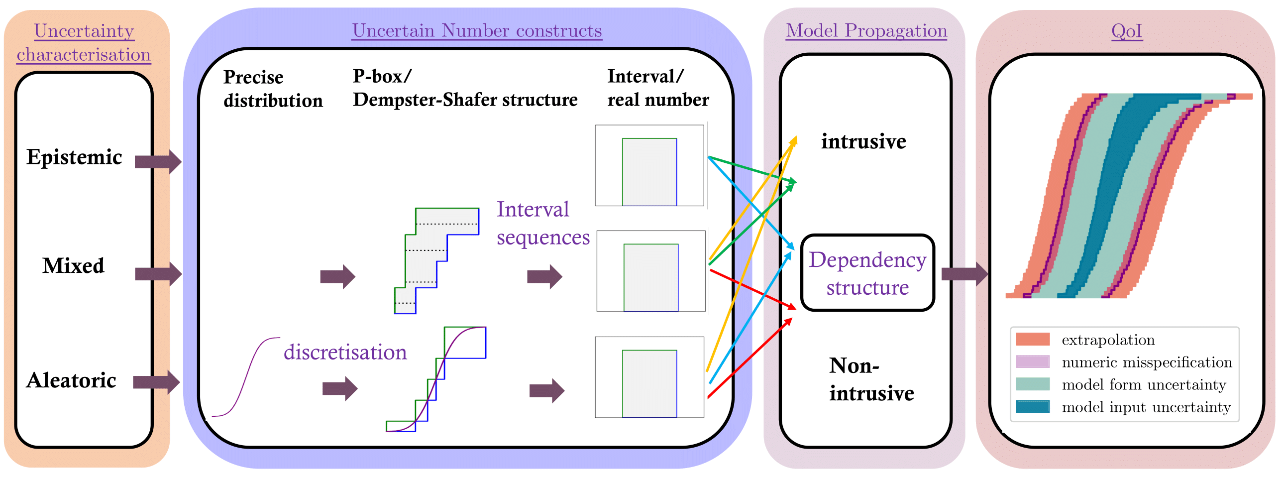
Figure 8:Flowchart of a comprehensive uncertainty analysis pipeline. Various dependency structures are denoted in colored arrows.
Figure 8 outlines a general computational pipeline typical for scientific numerical computations with a black-box model, which features the probability bounding approach during the stages of characterisation, propagation and finally the representation of QoI, and echos the idea that aleatory and epistemic uncertainty should be treated differently. Pairs of bounds constitute layered colour-shaded regions reflecting the sources of uncertainties involved. This provides a straightforward and intuitive way to account for the contributions of uncertainties in a comprehensive framework.
It should be noted that interval analysis plays a central role in the propagation of epistemic uncertainty and further mixed uncertainty or mixture of uncertainty. The slicing algorithm discretises a p-box into intervals and effectively propagate intervals. The same rigorous strategy also applies to precise distributions through outward-rounding.
Regarding the propagation methods for different types of uncertainty, various methods have been proposed, intrusive or nonintrusive, depending on the characteristic of the performance function such as linearity, monotonicity, or the accessibility to gradients.
Table 1 lists the characteristics of many methods.
Similar to the cases of information constraints for uncertainty characterisation, the more knowledge about the mathematical model, the higher chances of finding an efficient method.
Notably, enriched sampling methods such as nested Monte Carlo or interval Monte Carlo allows the outward (rigorous) implementation for a sampling signature consistent with aleatory uncertainty. This demonstrates the universal applicability and compatibility of sampling-based approaches for generic deterministic black-box models in scientific computing.
pyuncertainnumber provides high-level API to these methods and will automatically inspect the appropriateness of the propagating method given the characteristics of the function and uncertainty.
""" a typical workflow of uncertainty characterisation and propagation """
from pyuncertainnumber import Propagation

# constructions of uncertain number
a = pun.I(2, 3)
b = pun.normal(4, 1)
c = pun.uniform([4,5], [9,10])

# specify a response function
def foo(x): return x[0] ** 3 + 5 * x[1] + x[2]

# intrusive signature where uncertain numbers are drop-in replacements
response = foo([a, b, c])

# alternatively, to use a generic high-level propagation API
p = Propagation(vars=[a,b,c],
      func=foo,
      method='slicing',
      interval_strategy='direct'
)

# heavy-lifting of running propagation
response = p.run(n_slices=50)
Table 1:Characterisitics of uncertainty propagation methods
| uncertainty | Methods | cost | characteristics | Non-intrusive applicability |
|---|---|---|---|---|
| Aleatory | Monte Carlo methods | *** | Brute-force sampling | Yes |
| Taylor expansion | * | linearity assumption; gradient required | No | |
| Epistemic | interval arithmetic | * | vulnerable to dependency problem | No |
| Endpoints | ** | monotonicity over intervals; exponential growth | Yes | |
| Subinterval reconstitution | *** | computationally intensive with exponential growth | Yes | |
| Cauthy-Deviate method | *** | linearity assumption | Yes | |
| gradient-based optimisation | * | gradients required | No | |
| Gradient-free optimisation | *** | general applicability | Yes | |
| Mixed | Slicing | *** | transformed into interval propagation; cartesian product required | Yes |
| interval Monte Carlo | *** | general applicability with heavy cost; cartesian product required | Yes | |
| nested Monte Carlo | *** | double-loop sampling conditioned on epistemic variables; mixture of uncertainty | Yes |
3.3Uncertainty-aware surrogate models
Modern advanced numerical simulations are often computationally expensive, making abundant model evaluations required by uncertainty analysis impractical or even intractable. Surrogate models are therefore utilised to learn and generalise from observed data (a limited subset of DOE). Epistemic uncertainties exist not only in the model form (i.e. parameter and structure) but also in the extrapolation of predictions.
To account for such uncertainty, a probabilistic take of machine learning brings models that represent parameters in probability distributions (Bayesian neural networks), and models that represent a distribution of function structures (Gaussian Process). On the other hand, an intervalised or distribution-free view employs models that consider interval-valued parameters (Interval Predictor Model). These models have the prospects of efficiently propagating the input uncertainties to fully characterise the tail probability of the QoI for example in the imprecise reliability analysis (will be discussed in Section 4.1).
With many machine learning frameworks available in the Python ecosystem (e.g. Tensorflow, GPflow, PyIPM, etc), we provide the algorithms and the interface in pyuncertainnumber to extend those models to be combined within our framework to further propagate uncertain numbers for a efficient and comprehensive uncertainty management.
4Risk, reliability, and design optimisation under uncertainty
Uncertainty is often a means to an end for scientific computations. For example, risk assessment of environmental hazards (e.g. earthquakes), evaluation of performance and reliability of engineered system under uncertain environmental conditions, and supports of decision-makings for optimal engineering designs. An increasing acknowledgement of the mixture of uncertainty encountered in real world problems has led to the transition from the deterministic safety factor approach to probabilistic risk assessment, further to performance-based or reliability-based design protocols in several safety-critical industries Beer et al., 2013. A comprehensive and expressive uncertainty framework that reflects the contributions of various uncertainties is essential, and an accessible toolkit with universal uncertainty representations is beneficial in facilitating the adoption of comprehensive uncertainty management.
4.1Imprecise reliability analysis
Conventionally, in the analysis of a probabilistic safety framework, the probability of failure is given as which involves an integration of the joint probability distribution over the failure domain. Given the presence of epistemic uncertainty, the failure probability presents as an interval bound as opposed of precise probability measure. Consider a generic simulation in the face of mixed uncertainties such that the system variables cannot be precisely characterised but to be more appropriately modelled as an uncertain number, as suggested in Section 2. The interval of failure probability can be given as Zhang et al., 2010:
in which and denote the infimum and supremum function; Each uncertain number is discretised as pairs of focal elements and probability masses .
The computation of can be straightforwardly done by the methods discussed in Section 3.2 and pyuncertainnumber provides a simple function to easily evaluate the probability interval.
Figure 9 illustrates the conceptual comparison of expressing the probability of failure for both probabilistic and imprecise frameworks. Conventionally, the can be estimated using a Monte Carlo estimator that reads: , where denotes an indicator function, as shown in different colours in the histogram. This summation also depicts the blue cross in the empirical CDF in the top figure, where an interval of is shown in red.
![Illustration of failure probability \mathbb{P}[g(\boldsymbol{X}) \leq 0] for both probabilistic and imprecise frameworks where the probabilistic input is enclosed in the imprecise input](https://pub.curvenote.com/0199eb8c-c4ed-7079-8df8-bc8fe638155d/public/demon_pof_bounds-921e95525fb7fe47e5508d1169221782.png)
Figure 9:Illustration of failure probability for both probabilistic and imprecise frameworks where the probabilistic input is enclosed in the imprecise input
4.2Robust designs under epistemic and mixture of uncertainty
Considerable progress has been done towards design optimisation under uncertainty with a probabilistic framework. Typical formulations include robust optimisation aiming for designs less sensitive to variation and reliability-based optimisation whose constraints are less prone to failure under variability. However, real world scenarios commonly involve lack-of-knowledge uncertainties and, more often, mixture of uncertainties, which brings additional subtleties in the formulation. In recognition of the epistemic uncertainty, optimisation is directed with respect to an interval bound. As an example, Figure 10 shows a simple exemplar objective function assumed to represent the cost of manufacture, see (4), in the face of pure epistemic uncertainty.
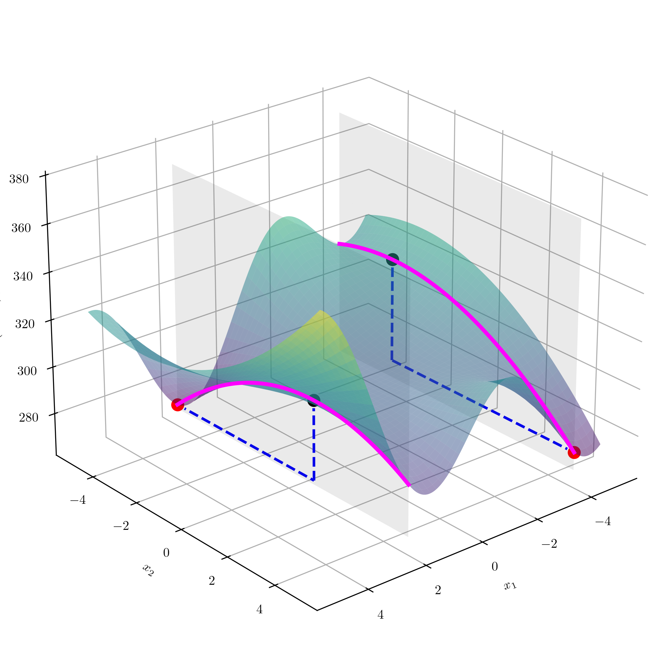
Figure 10:An examplar objective function. Two vertical planes corresponding to design variables and are shown, in which the intersecting curves as well as the maximum and minimum are specifically marked.
where denotes design variables of the range of , while denotes uncertain parameters. Given the pure epistemic uncertainty, a performance-oriented objective can be intuitively formulated as minimising the upper bound: , or a robustness-oriented objective which minimises the width the cost interval: .
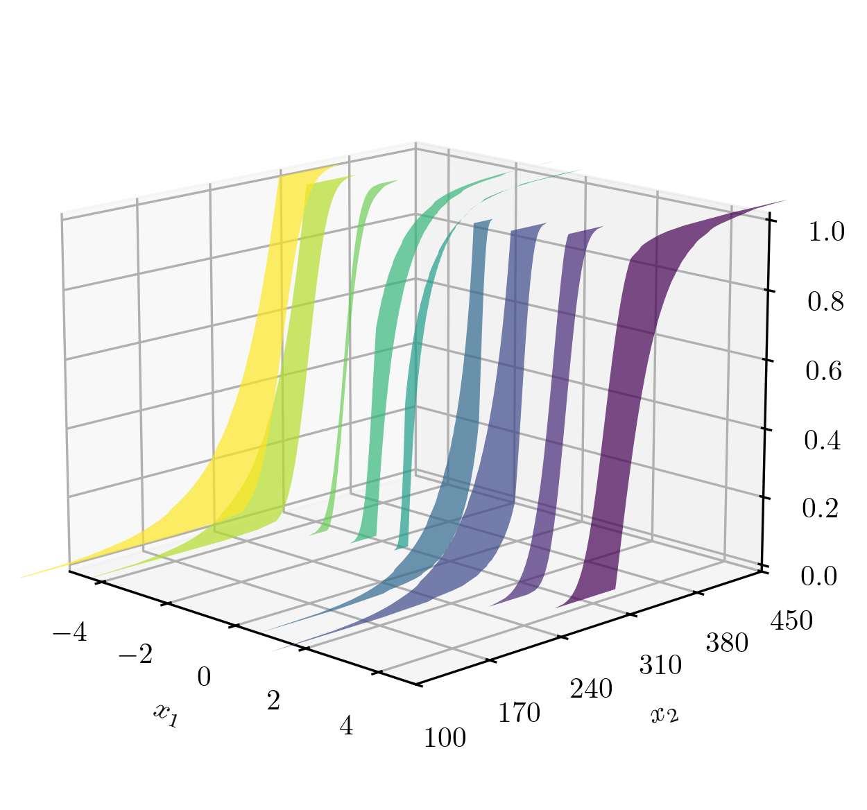
Figure 11:Illustration of the cost objective represented in uncertain numbers with respect to designs () in the face of mixed-type uncertain parameter ().
In mixed uncertainty cases, the cost w.r.t a design is effectively presented by p-boxes , as seen in Figure 11. The existence of epistemic domain results in a bounded objective such as an expected performance indicator or a probability measure, for which both operations will average out the aleatory space. Intuitively, in this example, one would desire to find the design accomplishing the minimum of the expected cost . Alternatively, it is also possible to prescribe the performance requirement in a probability statement as below, which optimises with the probability of having a cost higher than a prescribed budget , where .
This effectively introduces a constraint as to the budget. Note that upper bounds are used in the current formulation to take into effect of the epistemic uncertainty and to reflect a sense of performance guarantee. Additionally, to be more pragmatic, the objective can be compounded with another constraint which could for example reflects a cost-production tradeoff that a lower cost is aimed on the condition that a certain production requirement is probabilistically satisfied. An examplar formation can be given as follows where stands for extra constraint functions:
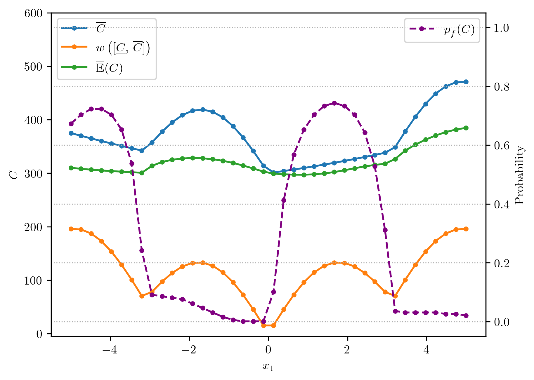
Figure 12:Optimisation tasks of different formulations in the face of mixed uncertainty
5Conclusion and Outlook
To know what you do not know suggests the importance to realise the assumptions and applicability of scientific computations to maximise the credibility for the resulting predictions, designs and decisions. Given the various sources of uncertainties and the often limited empirical information, how to appropriately represent, aggregate, propagate uncertainties is a critical challenge for trustworthy reliability and risk assessments, especially for safety critical applications. Current practices tend to go overboard with unjustified assumptions of Gaussianality and independence, mostly due to the computational simplicity and the lack of tools for a comprehensive uncertainty analysis. This leads to a need of a computational framework that effectively balances representational expressiveness and computational feasibility.
This paper presents the framework of uncertain number which fills this gap and presents several advantages:
(i) it is highly expressive enabling faithful characterisation of an uncertain quantity given various scenarios of partial knowledge where conventional probability theory struggles to cope;
(ii) it provides a closed environment where various characterisation, aggregation and propagation operations can be consistently conducted based on the unified structure, uncertain number;
(iii) it is underpinned by a probability bounding mechanism which intuitively showcases the notion of epistemic uncertainty --- wherein increased knowledge leads to progressively tighter bounds;
(iv) the bounding mechanism enables an explicit differentiation of aleatory and epistemic uncertainties, allowing their respective contributions to be accounted for during both characterisation and propagation.
The developed Python library, pyuncertainnumber, facilitates trustworthy management of uncertainty through faithful representation and rigorous propagation. Unlike other established Python-based general purpose uncertainty quantification (UQ) tools that primarily focus on probabilistic modelling -—- often requiring precise specification of distribution shape and dependency structures, which is challenging in practice in the face of partial information, pyuncertainnumber, however, relaxes such specification and is capable of rigorous treatment even with unknown knowledge states. It explicitly addresses both aleatory and epistemic uncertainty using appropriate methods without making unjustified assumptions, advancing uncertainty management to handle both variability and incertitude. Consequently, it enables a more robust framework for addressing real-world UQ challenges such as mixed uncertainty propagation and characterisation under partial knowledge.
As probabilistic programming provides support for automatic inference, we aim for an imprecise uncertainty analysis framework, where variables are consistently represented by uncertain numbers in the face of both variability and incertitude, allowing for extensions of deterministic functions to be computed in an automatic, comprehensive, and rigorous manner. Our next focus will be extending the framework of probabilistic programming, which has a heavy focus on Bayesian inference, into an imprecise realm where more comprehensive uncertainty structures can be integrated into the learning and inference of machine learning models.
This work has been supported by the DAWS2 (Development of Advanced Wing Solution 2) project funded by Innovate UK.
Copyright © 2025 Chen & Ferson. This is an open-access article distributed under the terms of the Creative Commons Attribution 4.0 International license, which enables reusers to distribute, remix, adapt, and build upon the material in any medium or format, so long as attribution is given to the creators.
pyuncertainnumberis a research-grade open-source library, with its source code available on GitHub and comprehesive documentation available online.also called randomness, aleatory uncertainty, objective uncertainty, dissonance, or irreducible uncertainty arised from natural stochasticity, environmental or structural variation across space or through time.
also called ignorance, epistemic uncertainty, non-specificity, or reducible uncertainty arised from incompleteness of knowledge.
the uncertain number could not be any tighter without more information.
- API
- application programming interface
- CDF
- cumulative distribution funcion
- CFD
- computational fluid dynamics
- DGM
- Data generating mechanism
- DOE
- design of experiments
- DSS
- Dempster Shafer structure
- i.i.d
- independent and identically distributed
- NLP
- natural language processing
- p-box
- probability boxes
- P-box
- probability boxes
- PBA
- probability bounds analysis
- QoI
- quantity of interest
- UQ
- uncertainty quantification
- Roy, C. J., & Oberkampf, W. L. (2011). A comprehensive framework for verification, validation, and uncertainty quantification in scientific computing. Computer Methods in Applied Mechanics and Engineering, 200(25–28), 2131–2144. https://doi.org/10.1016/j.cma.2011.03.016
- Oberkampf, W. L., Helton, J. C., Joslyn, C. A., Wojtkiewicz, S. F., & Ferson, S. (2004). Challenge problems: uncertainty in system response given uncertain parameters. Reliability Engineering & System Safety, 85(1–3), 11–19. 10.1016/j.ress.2004.03.002
- Smith, R. C. (2024). Uncertainty quantification: theory, implementation, and applications. SIAM. 10.1137/1.9781611973228
- Gray, A., Wimbush, A., de Angelis, M., Hristov, P. O., Calleja, D., Miralles-Dolz, E., & Rocchetta, R. (2022). From inference to design: A comprehensive framework for uncertainty quantification in engineering with limited information. Mechanical Systems and Signal Processing, 165, 108210. 10.1016/j.ymssp.2021.108210
- Beer, M., Ferson, S., & Kreinovich, V. (2013). Imprecise probabilities in engineering analyses. Mechanical Systems and Signal Processing, 37(1–2), 4–29. 10.1016/j.ymssp.2013.01.024
- Patelli, E., Broggi, M., Tolo, S., & Sadeghi, J. (2017). COSSAN SOFTWARE: A MULTIDISCIPLINARY AND COLLABORATIVE SOFTWARE FOR UNCERTAINTY QUANTIFICATION. Proceedings of the 2nd International Conference on Uncertainty Quantification in Computational Sciences and Engineering (UNCECOMP 2017), 212--224. 10.7712/120217.5364.16982
- Ferson, S., & Hajagos, J. G. (2004). Arithmetic with uncertain numbers: rigorous and (often) best possible answers. Reliability Engineering & System Safety, 85(1–3), 135–152. 10.1016/j.ress.2004.03.008
- Ferson, S., & Ginzburg, L. R. (1996). Different methods are needed to propagate ignorance and variability. Reliability Engineering & System Safety, 54(2–3), 133–144. 10.1016/s0951-8320(96)00071-3
- Destercke, S., Dubois, D., & Chojnacki, E. (2008). Unifying practical uncertainty representations–I: Generalized p-boxes. International Journal of Approximate Reasoning, 49(3), 649–663. 10.1016/j.ijar.2008.07.003
- Williamson, R. C., & Downs, T. (1990). Probabilistic arithmetic. I. Numerical methods for calculating convolutions and dependency bounds. International Journal of Approximate Reasoning, 4(2), 89--158. 10.1016/0888-613x(90)90022-t
- Ferson, S., Kreinovich, V., Ginzburg, L., Myers, D. S., & Sentz, K. (2003). Constructing probability boxes and Dempster-Shafer structures. Sandia National Laboratories. 10.2172/809606
- Gray, N., Ferson, S., De Angelis, M., Gray, A., & de Oliveira, F. B. (2022). Probability bounds analysis for Python. Software Impacts, 12, 100246. https://doi.org/10.1016/j.simpa.2022.100246
- Ferson, S., Kreinovich, V., Hajagos, J., Oberkampf, W. L., & Ginzburg, L. (2007). Experimental uncertainty estimation and statistics for data having interval uncertainty. [Techreport]. Sandia National Laboratories (SNL), Albuquerque, NM,. 10.2172/910198
- de Angelis, M. (2022). intervals (v0.1) [Computer software]. Zenodo. 10.5281/zenodo.6205624
- Tretiak, K., & Ferson, S. (2023). Should data ever be thrown away? Pooling interval-censored data sets with different precision. International Journal of Approximate Reasoning, 156, 114–133. 10.1016/j.ijar.2023.02.007
