Imprecise uncertainty management with uncertain numbers to facilitate trustworthy computations

Yu Chen; Scott Ferson

doi:10.25080/ahrt5264

Tutorial: a workflow of uncertainty characterisation, aggregation, and propagation using pyuncertainnumber

,

1setup¶

1.1Installation¶

Install the pyuncertainnumber library from PyPI.

pip install pyuncertainnumber

Important

A virtual enviroment is recommended for installation.

Follow the instructions for additional details to install pyuncertainnumber.

from pyuncertainnumber import UN
import pyuncertainnumber as pun
import numpy as np
import matplotlib.pyplot as plt

# set up a global plotting style
plt.rcParams.update({
        "font.size": 11,
        "text.usetex": True,
        "font.family": "serif",
        "legend.fontsize": 'small',
        })

2Characterisation¶

2.1Canonical specification¶

There are two ways to specify an uncertain number when you have enough information: a verbose way to specify all the fields and a shortcut way to focus on computational purposes. Later sections will show many situations where you have only partial information.

Tip

When specifying intervals, whether directly for an interval-type uncertain number or interval-valued shape parameters in a p-box, one can use natual language such as “about 3”, “around 3” or intuitive format ‘[3 +- 10%]’.
Also, one can explicitly call using argument essence=‘pbox’ or implicitly call distribution with interval parameters
There are many more fields avilable to portrait the modelled uncertain quantify, such as “provenence”, “justification”, etc.

# verbose specification of uncertain numbers
# interval-type uncertain number
a = UN(name='elas_modulus', 
                 symbol='E', 
                 units='Pa', 
                 essence='interval', 
                 intervals=[2,3]
                )

# distribution-type uncertain number
b = UN(
    name='elas_modulus', 
    symbol='E', 
    units='Pa', 
    essence='distribution', 
    distribution_parameters=['gaussian', (6, 2)])

# pbox-type uncertain number
c = UN(
    name='elas_modulus', 
    symbol='E', 
    units='Pa', 
    essence='pbox', 
    distribution_parameters=['gaussian', ([0,12],[1,4])])

# dempster-shafer-type uncertain number
d = UN(
    name='elas_modulus', 
    symbol='E', 
    units='Pa', 
    essence='dempster_shafer', 
    intervals=[[1,5], [3,6]], 
    masses=[0.5, 0.5]
    )

fig, (ax1, ax2, ax3, ax4) = plt.subplots(ncols=4, figsize=(18, 3))
a.plot(ax=ax1, title='Interval-type uncertain number')
b.plot(ax=ax2, title='distribution-type uncertain number')
c.plot(ax=ax3, title='p-box type uncertain number', nuance='curve')
d.plot(ax=ax4, title='DSS-type uncertain number', nuance='curve')
plt.show()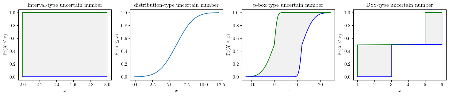

Important

Alternatively, shortcuts existed to instantiate uncertain numbers are also possible when one wants to quickly get on with calculations.

# shortcuts to instantiate uncertain numbers
a = pun.I(2, 3)
b = pun.D('gaussian', (6, 2))
c = pun.normal([0,12], [1,4])
d = pun.DSS([[1,5], [3,6]], [0.5, 0.5])

2.2Known constraints¶

Often there is only partial empirical information (e.g. statistical information) pertaining some variables. A faithful characterisation entails that all of the available statistical information should be utilised but without introducing any extra assumptions beyond what are empirically justified.

fig, axes = plt.subplots(nrows=1, ncols=4, figsize=(12, 3), layout="constrained")
pun.known_constraints(mean=0, var=0.25).plot(title='MeanVar(0, 0.25)', ax=axes[0], nuance='curve')
pun.known_constraints(minimum=0, mean=1).plot(title='MeanMin(1,0)', ax=axes[1], nuance='curve')
pun.known_constraints(minimum=0, mean=1, maximum=2).plot(title='MeanMinMax(1,0,2)', ax=axes[2], nuance='curve')
pun.known_constraints(minimum=0, mean=1, var=0.25, maximum=2).plot(title='MinMaxMeanVar(0, 2, 1, 0.25)', ax=axes[3], nuance='curve')
plt.show()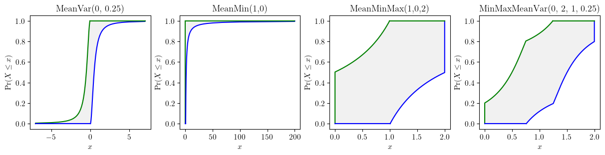

2.3Characterisation from empirical measurements¶

Empirical data rarely come in perfect forms, especially for in situ measurements. Practical computations frequently deal with poor measurements. Data uncertainty mainly consists of sampling uncertainty and measurement uncertainty. Both parametric and nonparametric estimators are provided to characterise data uncertainties.

from pyuncertainnumber import pba
import scipy.stats as sps

precise_sample = sps.expon(scale=1/0.4).rvs(15)
imprecise_data = pba.I(lo = precise_sample - 1.4, hi=precise_sample + 1.4)

# parametric estimator
fn = pun.fit('mom', family='exponential', data=imprecise_data)
fn.display(title='fitted exponential p-box with imprecise data', nuance='curve')

# nonparametric estimator with the KS bounds 
b_l, b_r = pun.KS_bounds(imprecise_data, alpha=0.025, display=True)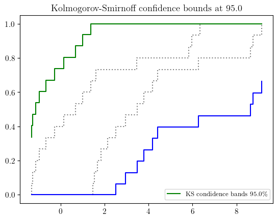

3Aggregation of various sources of information, expert elicitation, or evidence¶

from pyuncertainnumber import stochastic_mixture, envelope
from pyuncertainnumber.pba.ecdf import pl_ecdf_bounding_bundles
from pyuncertainnumber.pba.dss import plot_DS_structure_with_labels

3.1expert elicitation is represented as probability distribution¶

a_d = pun.D('gaussian', (-5, 2))
b_d = pun.D('normal', (1.5, 3.))
c_d = pun.D('uniform', (1, 12))
d_d = pun.D('gaussian', (10, 1.5))
fixed_value=0
p_env = envelope(a_d, b_d, c_d, d_d)

fig, ax = plt.subplots(figsize=(4, 3))
a_d.plot(ax=ax, label='expert a', color='green', ls='--', zorder=100)
b_d.plot(ax=ax, color='salmon', zorder=50, ls='--', label='expert b')
c_d.plot(ax=ax, label='expert c', color='purple', ls='--', zorder=100)
d_d.plot(ax=ax, label='expert d', color='blue', ls='--', zorder=100)
ax.vlines(fixed_value, ymin=0, ymax=1, color='black', linestyle='dashdot', label='expert e')
p_env.plot(ax=ax,  bound_colors=['lightgray', 'lightgray'], fill_color='lightgray', label='envelope p-box')
ax.set_title("envelope aggregation of expert elicitations")
ax.legend(loc="center left", bbox_to_anchor=(1, 0.5))
plt.show()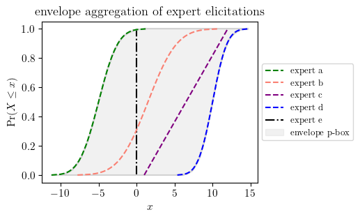

3.2expert opinion is represented as intervals¶

a = pun.I(1,5)
b = pun.I(3,6)
c = pun.I(2,3)
d = pun.I(2,9)

dss = stochastic_mixture(a,b,c,d)

fig, (ax0, ax1) = plt.subplots(ncols=2, figsize=(8, 3))                          
ax0 = plot_DS_structure_with_labels([a,b,c,d], masses=[0.25, 0.25, 0.25, 0.25], offset=1.5, ax=ax0)
dss.plot(ax=ax1)
plt.show()

4Uncertainty propagation¶

4.1arithmetic of uncertain number¶

Probability bounds anlaysis combines both interval analysis and probability theory, allowing rigorous bounds of (arithmetic) functions of random variables to be computed even with partial information.

X = pun.uniform(1, [2,3])
Y = X

fig, axes = plt.subplots(nrows=2, ncols=4, sharey=True, figsize=(12, 6), layout="constrained")

X.plot(ax=axes[0, 0], title='$X, Y \sim U(1, [2,3])$', nuance='curve')

# add Perfect
Z_add_p = X.mul(Y, dependency='p')
Z_add_p.plot(ax=axes[0, 1], title='X+Y Perfect', fill_color='lightblue', nuance='curve')

# mul Opposite
Z_mul_o = X.mul(Y, dependency='o')
Z_mul_f = X.mul(Y, dependency='f')
Z_mul_f.plot(ax=axes[1, 0], title="X × Y Fréchet", fill_color='red', nuance='curve')

# div Independence
Z_div_i = X.div(Y, dependency='i')
Z_div_f = X.div(Y, dependency='f')
Z_div_i.plot(ax=axes[1, 1], title='X/Y Independence', fill_color='orange', nuance='curve')

### unary ops ###
# squared
(X**0.5).plot(ax=axes[0,2], title='$\sqrt{X}$', nuance='curve')

# exponential
X.exp().plot(ax=axes[0,3], title='$e^{X}$', nuance='curve')

# sin
X.sin().plot(ax=axes[1,2], title='$\sin(X)$', nuance='curve')

# tanh
X.tanh().plot(ax=axes[1,3], title=r"$\tanh (X)$", nuance='curve')

plt.show()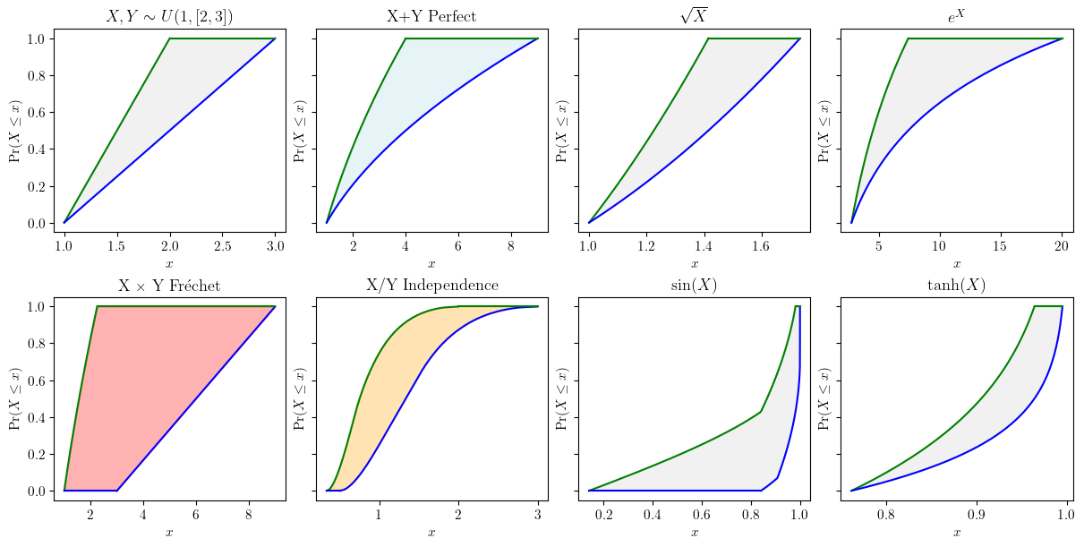

Note

Beyond arithmetics, various advanced methods have been proposed for propagation of diﬀerent types of uncertainties, intrusive or nonintrusive, depending on the characteristic of the performance function such as linearity, monotonicity, or the accessibility to gradients. See additional details in the documentation.

A high-level API has been provided for delpoying these various methods under various uncertainty situations with a consistent signature.

4.2generic propagation of uncertain numbers¶

from pyuncertainnumber import Propagation

a = pun.I(2, 3)
b = pun.normal(10, 1)
c = pun.normal([6, 9], 3)

# specify a response function
def foo(x):  
    if isinstance(x, np.ndarray):
        if x.ndim == 1:
            x = x[None, :]
        return x[:, 0] ** 3 + x[:, 1] + x[:, 2]# vectorised signature
    else:
        return x[0] ** 3 + x[1] + x[2]  # iterable signature

# intrusive call signature as drop-in replacements
response = foo([a, b, c])

response.display()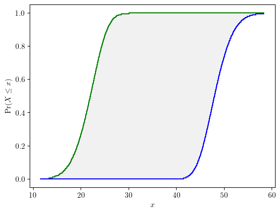

# a generic call signature
p = Propagation(vars=[a, b, c], func=foo, method='slicing', interval_strategy='subinterval')
response = p.run(n_slices=50, n_sub=2, style='endpoints')

INFO: mixed uncertainty propagation

Warning

The computational cost increases exponentially with the number of input variables and the number of slices. Be cautious with the choice of number of slices n_slices given the number of input variables of the response function.

response.display()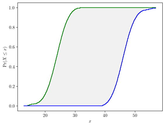

License¶

Copyright © 2025 Chen & Ferson. This is an open-access article distributed under the terms of the Creative Commons Attribution 4.0 International license, which enables reusers to distribute, remix, adapt, and build upon the material in any medium or format, so long as attribution is given to the creators.

Abbreviations¶

API: application programming interface
p-box: probability boxes