
This notebook contains the code for the SHAP analysis for a Gradient Boosted Decision Tree (GBDT) model.
Required libraries:
ucimlrepo
xgboost
shap
matplotlib
scikit-learn
pandas
numpy
import warnings
import numpy as np
import pandas as pd
import matplotlib.pyplot as plt
from xgboost import XGBClassifier
from sklearn.model_selection import train_test_split
import shap
from sklearn.metrics import RocCurveDisplay


warnings.filterwarnings("ignore", category=FutureWarning)
TEST_SIZE = 0.2
RANDOM_STATE = 421Load the Data
from ucimlrepo import fetch_ucirepo

# fetch dataset
bank_marketing = fetch_ucirepo(id=222)

# data (as pandas dataframes)
X = bank_marketing.data.features
y = bank_marketing.data.targets
# variable information
bank_marketing.variables.head() name role type demographic \
0 age Feature Integer Age
1 job Feature Categorical Occupation
2 marital Feature Categorical Marital Status
3 education Feature Categorical Education Level
4 default Feature Binary None
description units missing_values
0 None None no
1 type of job (categorical: 'admin.','blue-colla... None no
2 marital status (categorical: 'divorced','marri... None no
3 (categorical: 'basic.4y','basic.6y','basic.9y'... None no
4 has credit in default? None no print("X shape: ", X.shape)
print("y shape: ", y.shape)X shape: (45211, 16)
y shape: (45211, 1)
2Preprocess Dataset
2.1Convert the target variable to numeric
y = y.replace({"no": 0, "yes": 1})
y.value_counts()
y
0 39922
1 5289
Name: count, dtype: int642.2Drop the duration column
The duration of the call is not available before the call is made, and hence cannot be used for prediction.
X = X.drop(columns=["duration"])2.3Convert categorical features to categorical datatype
obj_cols = X.select_dtypes(include="object").columns
for c in obj_cols:
    X[c] = pd.Categorical(X[c])
print("Number of categorical features: ", len(obj_cols))
Number of categorical features: 9
2.4Split dataset into train and test sets
x_train, x_test, y_train, y_test = train_test_split(
    X, y, test_size=TEST_SIZE, random_state=RANDOM_STATE
)
print(x_train.shape, x_test.shape, y_train.shape, y_test.shape)
(36168, 15) (9043, 15) (36168, 1) (9043, 1)
3Train model
xgb = XGBClassifier(enable_categorical=True)
xgb.fit(x_train, y_train)
XGBClassifier(base_score=None, booster=None, callbacks=None,
colsample_bylevel=None, colsample_bynode=None,
colsample_bytree=None, device=None, early_stopping_rounds=None,
enable_categorical=True, eval_metric=None, feature_types=None,
feature_weights=None, gamma=None, grow_policy=None,
importance_type=None, interaction_constraints=None,
learning_rate=None, max_bin=None, max_cat_threshold=None,
max_cat_to_onehot=None, max_delta_step=None, max_depth=None,
max_leaves=None, min_child_weight=None, missing=nan,
monotone_constraints=None, multi_strategy=None, n_estimators=None,
n_jobs=None, num_parallel_tree=None, ...)4Evaluate
ax = plt.gca()
ax.grid(True)
ax.set_title("ROC Curve for XGBoost Classifier on the Test Set")
_ = RocCurveDisplay.from_estimator(
    xgb, x_test, y_test, ax=ax, name="XGBoost Classifier"
)
plt.tight_layout()
ax.set_xlabel("False Positive Rate: (Positive Class: yes)")
ax.set_ylabel("True Positive Rate: (Positive Class: yes)")
# plt.savefig("../roc_xgb.png")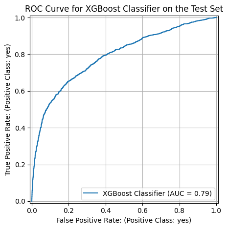
print("Train accuracy: ", xgb.score(x_train, y_train))
print("Test accuracy: ", xgb.score(x_test, y_test))
Train accuracy: 0.9355784118557842
Test accuracy: 0.8917394669910428
5SHAP Analysis
shap.initjs()<IPython.core.display.HTML object>explainer = shap.TreeExplainer(xgb)
shap_values = explainer(x_test)
shap_values.shape(9043, 15)5.1Global Explanations
5.1.1Bar Plot
shap.plots.bar(shap_values)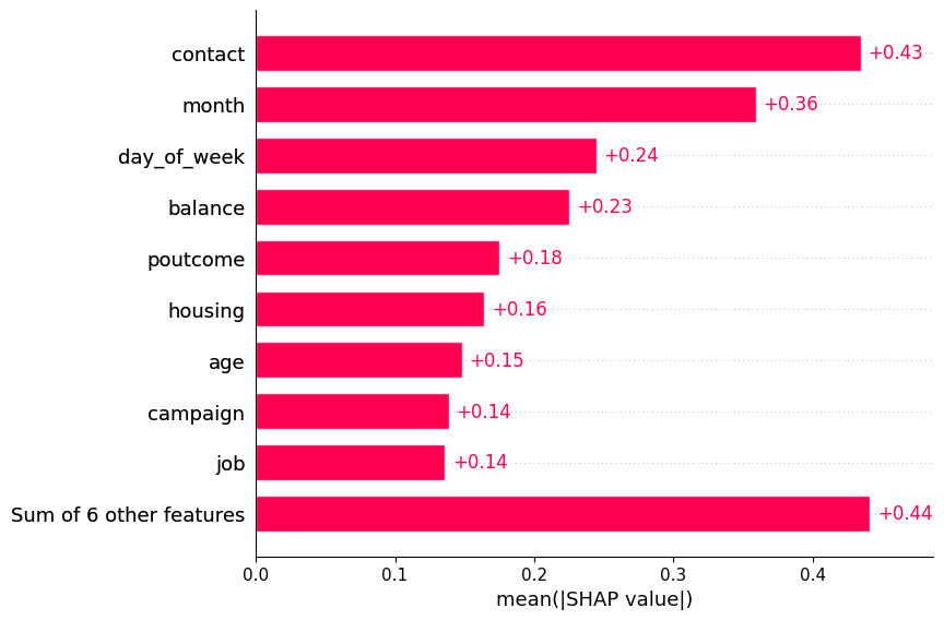
5.1.2Beeswarm Plot
ax = plt.subplot()
ax.grid(True)
ax = shap.plots.beeswarm(shap_values, max_display=16, show=False, log_scale=False)
ax.set_title("Global SHAP Values for XGBoost Classifier")
plt.tight_layout()
# plt.savefig("../beeswarm_xgb.png")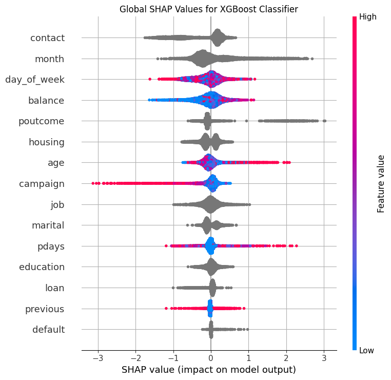
5.2Dependency Explanations
def plot_shap_categorical(
    shap_values: shap.Explanation,
    x: pd.DataFrame,
    feature_name: str,
    save_path: str = None,
) -> plt.Axes:
    """Plot SHAP dependence plot for a categorical feature.

    Args:
        shap_values (shap.Explanation): SHAP values for the test set.
        x (pd.DataFrame): Test set.
        feature_name (str): Name of the categorical feature.
        save_path (str, optional): Path to save the plot. Defaults to None.

    Returns:
        plt.Axes: Axes object for the plot.
    """
    feature_idx = x.columns.tolist().index(feature_name)
    feature_values = x.iloc[:, feature_idx]
    shap_values_feature = shap_values[:, feature_idx].values

    # Map categories to numeric values for plotting
    categories = feature_values.unique()
    category_to_num = {cat: num for num, cat in enumerate(categories)}
    feature_values_numeric = feature_values.map(category_to_num)

    # Create scatter plot with categories on x-axis
    _, ax = plt.subplots(figsize=(10, 6))
    # plt.figure(figsize=(10, 6))
    ax.scatter(
        feature_values_numeric,
        shap_values_feature,
        alpha=0.7,
        s=120,
    )

    # Replace numeric x-ticks with category labels
    ax.set_xticks(
        ticks=np.arange(len(categories)), labels=categories, rotation=45, fontsize=12
    )

    # Reference line at y=0
    ax.axhline(y=0, color="gray", linestyle="--")

    # Labels and title
    ax.grid(True)
    ax.set_xlabel(f"Categorical Feature: {feature_name}")
    ax.set_ylabel("SHAP Value")
    ax.set_title(f"SHAP Dependence Plot for Categorical Feature '{feature_name}'")

    plt.tight_layout()
    if save_path:
        plt.savefig(save_path)
    return ax
ax = plot_shap_categorical(shap_values, x_test, "poutcome", "../dep_poutcome_xgb.png")
ax = plot_shap_categorical(shap_values, x_test, "marital")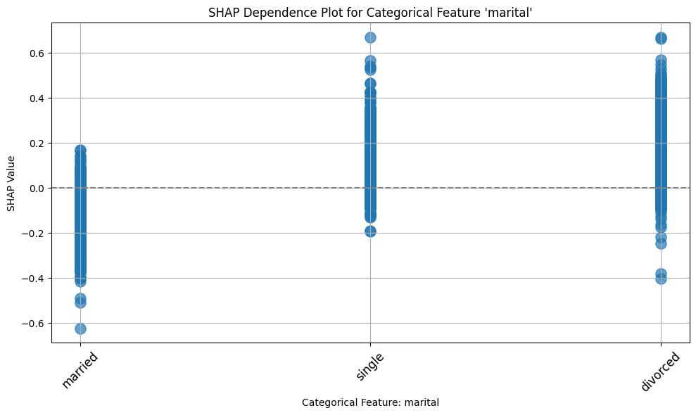
ax = plot_shap_categorical(shap_values, x_test, "education")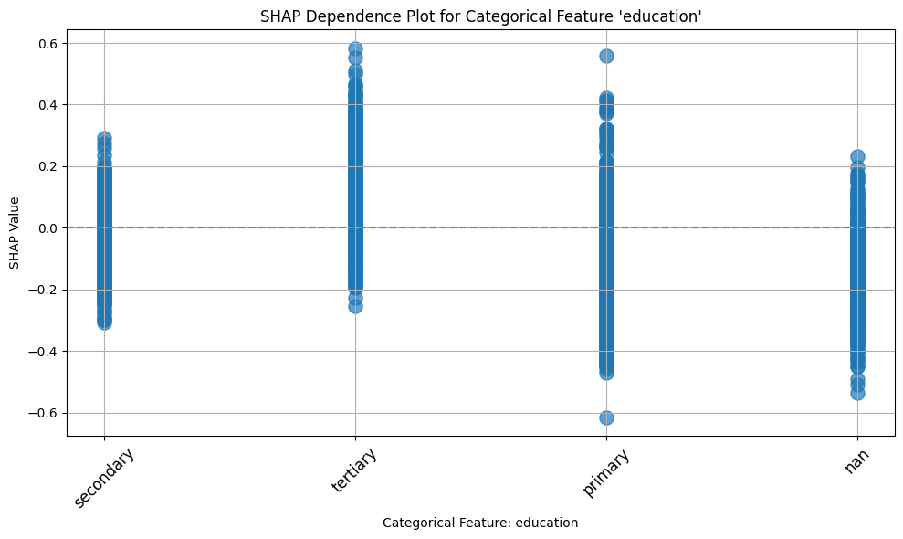
ax = plot_shap_categorical(shap_values, x_test, "job")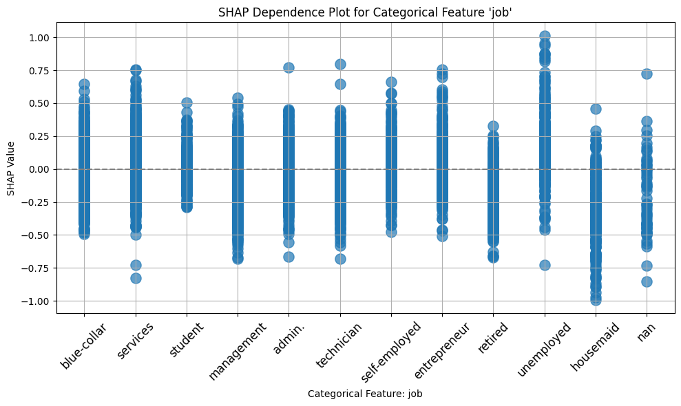
ax = plot_shap_categorical(shap_values, x_test, "default")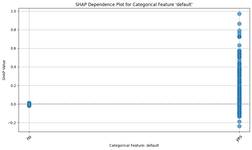
ax2 = plot_shap_categorical(shap_values, x_test, "housing")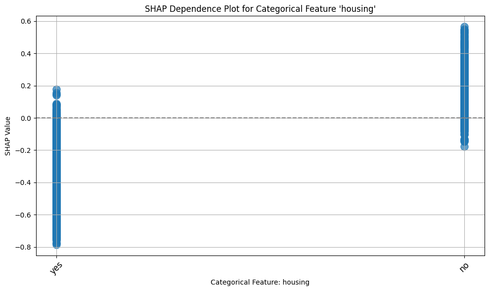
def plot_shap_dependence_subplots(
    features: list[str],
    xgb_model: XGBClassifier,
    shap_values: shap.Explanation,
    x_test: pd.DataFrame,
):
    """
    Plot SHAP dependence plots for multiple categorical features in subplots.

    Args:
        features (list[str]): List of feature names to plot.
        xgb_model (XGBClassifier): Trained XGBoost model.
        shap_values (shap.Explanation): SHAP values for the test set.
        x_test (pd.DataFrame): Test set.
    """
    num_features = len(features)
    cols = 2
    rows = (num_features + 1) // cols

    fig, axes = plt.subplots(rows, cols, figsize=(12, 4 * rows))

    for i, feature_name in enumerate(features):
        ax = axes.flatten()[i]

        feature_idx = xgb_model.feature_names_in_.tolist().index(feature_name)
        feature_values = x_test.iloc[:, feature_idx]
        shap_values_feature = shap_values[:, feature_idx].values

        categories = feature_values.unique()
        category_to_num = {cat: num for num, cat in enumerate(categories)}
        feature_values_numeric = feature_values.map(category_to_num)

        ax.scatter(
            feature_values_numeric,
            shap_values_feature,
            alpha=0.7,
            s=50,
            color="dodgerblue",
        )

        ax.axhline(y=0, color="gray", linestyle="--")
        ax.set_xticks(np.arange(len(categories)))
        ax.set_xticklabels(categories, rotation=45)
        ax.set_xlabel(f"{feature_name}")
        ax.set_ylabel("SHAP Value")
        ax.set_title(f"SHAP Dependence: {feature_name}")
        ax.grid(True)

    # Remove any unused subplots
    if num_features < rows * cols:
        for j in range(num_features, rows * cols):
            fig.delaxes(axes.flatten()[j])

    fig.tight_layout()
features = ["housing", "education", "marital", "poutcome"]
plot_shap_dependence_subplots(
features, xgb_model=xgb, shap_values=shap_values, x_test=x_test
)
plt.savefig("../dep_categorical_xgb.png")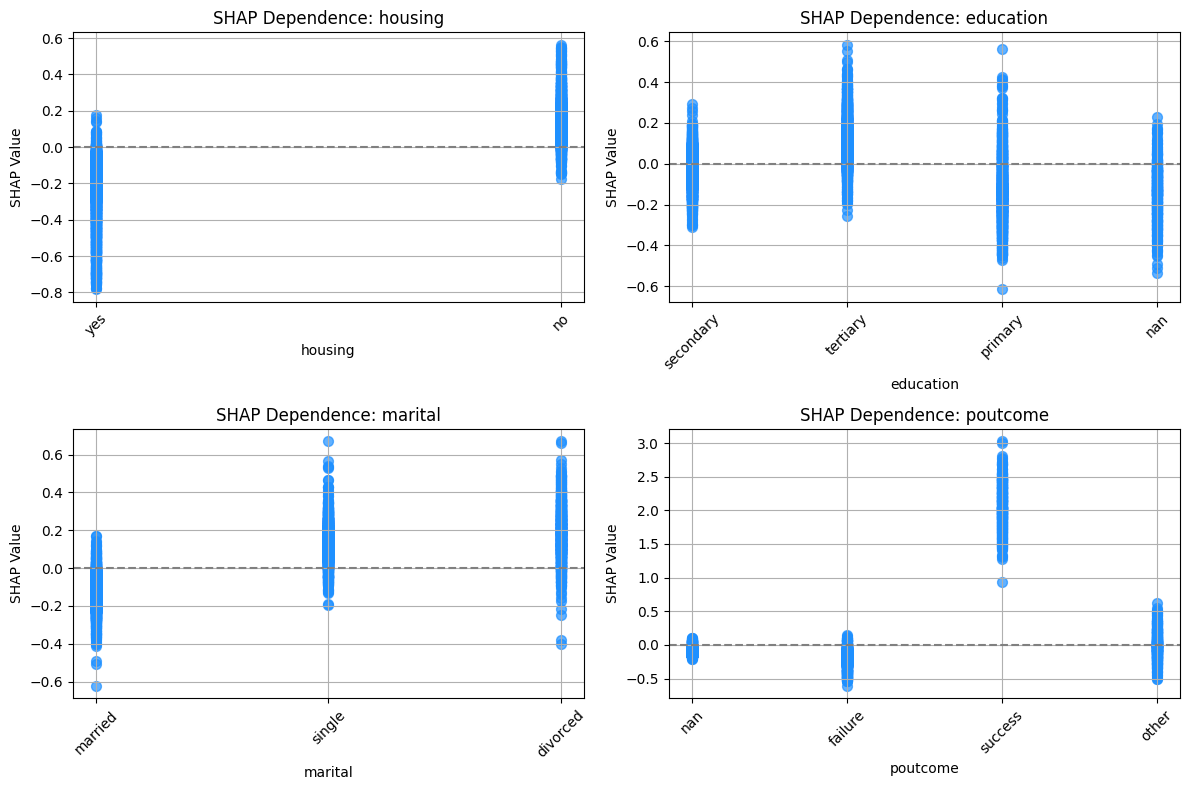
Copyright © 2025 Basu. This is an open-access article distributed under the terms of the Creative Commons Attribution 4.0 International license, which enables reusers to distribute, remix, adapt, and build upon the material in any medium or format, so long as attribution is given to the creator.
- GBDT
- Gradient Boosted Decision Trees
- SHAP
- SHapley Additive exPlanations